Authors: Michio Kaku,Robert O'Keefe
Hyperspace (8 page)

Riemann spent several months recovering from his nervous breakdown. Finally, when he delivered his oral presentation in 1854, the reception was enthusiastic. In retrospect, this was, without question, one of the most important public lectures in the history of mathematics. Word spread quickly throughout Europe that Riemann had decisively broken out of the confines of Euclidean geometry that had ruled mathematics for 2 millennia. News of the lecture soon spread throughout all the centers of learning in Europe, and his contributions to mathematics were being hailed throughout the academic world. His talk was translated into several languages and created quite a sensation in mathematics. There was no turning back to the work of Euclid.
Like many of the greatest works in physics and mathematics, the essential kernel underlying Riemann’s great paper is simple to understand. Riemann began with the famous Pythagorean Theorem, one of the Greeks’ greatest discoveries in mathematics. The theorem establishes the relationship between the lengths of the three sides of a right triangle: It states that the sum of the squares of the smaller sides equals the square of the longest side, the hypotenuse; that is, if
a
and
b
are the lengths of the two short sides, and
c
is the length of the hypotenuse, then
a
2
+
b
2
=
c
2
. (The Pythagorean Theorem, of course, is the foundation of all architecture; every structure built on this planet is based on it.)
For three-dimensional space, the theorum can easily be generalized. It states that the sum of the squares of three adjacent sides of a cube is equal to the square of the diagonal; so if
a, b
, and
c
represent the sides of a cube, and
d
is its diagonal length, then
a
2
+
b
2
+
c
2
=
d
2
(
Figure 2.1
).
It is now simple to generalize this to the case of
N
-dimensions. Imagine an
N
-dimensional cube. If
a, b, c
, … are the lengths of the sides of a “hypercube,” and
z
is the length of the diagonal, then
a
2
+
b
2
+
c
2
+
d
2
+ … =
z
2
. Remarkably, even though our brains cannot visualize an
N
-dimensional cube, it is easy to write down the formula for its sides. (This is a common feature of working in hyperspace. Mathematically manipulating
N
-dimensional space is no more difficult than manipulating three-dimensional space. It is nothing short of amazing that on a plain sheet of paper, you can mathematically describe the properties of higher-dimensional objects that cannot be visualized by our brains.)

Figure 2.1. The length of a diagonal of a cube is given by a three-dimensional version of the Pythagorean Theorem:
a
2
+ b
2
+ c
2
= d
2
.
By simply adding more terms to the Pythagorean Theorem, this equation easily generalizes to the diagonal of a hypercube in
N
dimensions. Thus although higher dimensions cannot be visualized, it is easy to represent
N
dimensions mathematically
.
Riemann then generalized these equations for spaces of arbitrary dimension. These spaces can be either flat or curved. If flat, then the usual axioms of Euclid apply: The shortest distance between two points is a straight line, parallel lines never meet, and the sum of the interior angles of a triangle add to 180 degrees. But Riemann also found that surfaces can have “positive curvature,” as in the surface of a sphere, where parallel lines always meet and where the sum of the angles of a triangle can exceed 180 degrees. Surfaces can also have “negative curvature,”
as in a saddle-shaped or a trumpet-shaped surface. On these surfaces, the sum of the interior angles of a triangle add to less than 180 degrees. Given a line and a point off that line, there are an infinite number of parallel lines one can draw through that point (
Figure 2.2
).
Riemann’s aim was to introduce a new object in mathematics that would enable him to describe all surfaces, no matter how complicated. This inevitably led him to reintroduce Faraday’s concept of the field.
Faraday’s field, we recall, was like a farmer’s field, which occupies a region of two-dimensional space. Faraday’s field occupies a region of three-dimensional space; at any point in space, we assign a collection of numbers that describes the magnetic or electric force at that point. Riemann’s idea was to introduce a collection of numbers at every point in space that would describe how much it was bent or curved.
For example, for an ordinary two-dimensional surface, Riemann introduced a collection of three numbers at every point that completely describe the bending of that surface. Riemann found that in four spatial dimensions, one needs a collection of ten numbers at each point to describe its properties. No matter how crumpled or distorted the space, this collection of ten numbers at each point is sufficient to encode all the information about that space. Let us label these ten numbers by the symbols g
11
, g
12
, g
13
,…. (When analyzing a four-dimensional space, the lower index can range from one to four.) Then Riemann’s collection of ten numbers can be symmetrically arranged as in
Figure 2.3
.
7
(It appears as though there are 16 components. However, g
12
= g
21
, g
13
= g
31
, and so on, so there are actually only ten independent components.) Today, this collection of numbers is called the Riemann
metric tensor
. Roughly speaking, the greater the value of the metric tensor, the greater the crumpling of the sheet. No matter how crumpled the sheet of paper, the metric tensor gives us a simple means of measuring its curvature at any point. If we flattened the crumpled sheet completely, then we would retrieve the formula of Pythagoras.
Riemann’s metric tensor allowed him to erect a powerful apparatus for describing spaces of any dimension with arbitrary curvature. To his surprise, he found that all these spaces are well defined and self-consistent. Previously, it was thought that terrible contradictions would arise when investigating the forbidden world of higher dimensions. To his surprise, Riemann found none. In fact, it was almost trivial to extend his work to
N
-dimensional space. The metric tensor would now resemble the squares of a checker board that was N × N in size. This will have profound physical implications when we discuss the unification of all forces in the next several chapters.

Figure 2.2. A plane has zero curvature. In Euclidean geometry, the interior angles of a triangle sum to 180 degrees, and parallel lines never meet. In non-Euclidean geometry, a sphere has positive curvature. A triangle’s interior angles sum to greater than 180 degrees and parallel lines always meet. (Parallel lines include arcs whose centers coincide with the center of the sphere. This rules out latitudinal lines.) A saddle has negative curvature. The interior angles sum to less than 180 degrees. There are an infinite number of lines parallel to a given line that go through a fixed point
.

Figure 2.3. Riemann’s metric tensor contains all the information necessary to describe mathematically a curved space in
N
dimensions. It takes 16 numbers to describe the metric tensor for each point in four-dimensional space. These numbers can be arranged in a square array (six of these numbers are actually redundant; so the metric tensor has ten independent numbers)
.
(The secret of unification, we will see, lies in expanding Riemann’s metric to
N-
dimensional space and then chopping it up into rectangular pieces. Each rectangular piece corresponds to a different force. In this way, we can describe the various forces of nature by slotting them into the metric tensor like pieces of a puzzle. This is the mathematical expression of the principle that higher-dimensional space unifies the laws of nature, that there is “enough room” to unite them in
N
-dimensional space. More precisely, there is “enough room” in Riemann’s metric to unite the forces of nature.)
Riemann anticipated another development in physics; he was one of the first to discuss multiply connected spaces, or wormholes. To visualize this concept, take two sheets of paper and place one on top of the other. Make a short cut on each sheet with scissors. Then glue the two sheets together along the two cuts (
Figure 2.4
). (This is topologically the same as
Figure 1.1
, except that the neck of the wormhole has length zero.)
If a bug lives on the top sheet, he may one day accidentally walk into the cut and find himself on the bottom sheet. He will be puzzled because everything is in the wrong place. After much experimentation, the bug will find that he can re-emerge in his usual world by re-entering the cut. If he walks around the cut, then his world looks normal; but when he tries to take a short-cut through the cut, he has a problem.
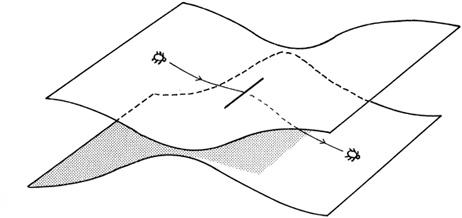
Figure 2.4. Riemann ’s cut, with two sheets are connected together along a line. If we walk around the cut, we stay within the same space. But if we walk through the cut, we pass from one sheet to the next. This is a multiply connected surface
.
Riemann’s cuts are an example of a wormhole (except that it has zero length) connecting two spaces. Riemann’s cuts were used with great effect by the mathematician Lewis Carroll in his book
Through the Looking-Glass
. Riemann’s cut, connecting England with Wonderland, is the looking glass. Today, Riemann’s cuts survive in two forms. First, they are cited in every graduate mathematics course in the world when applied to the theory of electrostatics or conformal mapping. Second, Riemann’s cuts can be found in episodes of “The Twilight Zone.” (It should be stressed that Riemann himself did not view his cuts as a mode of travel between universes.)