101 Excel 2013 Tips, Tricks and Timesavers (21 page)
Read 101 Excel 2013 Tips, Tricks and Timesavers Online
Authors: John Walkenbach

Figure 50-1:
Using the INDIRECT function to sum user-specified rows.
The argument for the INDIRECT function uses the concatenation operator to build a range reference by using the values in cells E2 and E3. So, if E2 contains 2 and E3 contains 4, the range reference evaluates to this string:
“B2:B4”
The INDIRECT function converts that string to an actual range reference, which is then passed to the SUM function. In effect, the formula returns
=SUM(B2:B4)
When you change the values in E2 or E3, the formula is updated to display the sum of the specified rows.
Specifying worksheet names indirectly
Figure 50-2 shows another example, this time using a worksheet reference.
Column A, on the Summary worksheet, contains text that corresponds to other worksheets in the workbook. Column B contains formulas that reference these text items. For example, the formula in cell B2 is
=SUM(INDIRECT(A2&”!F1:F10”))
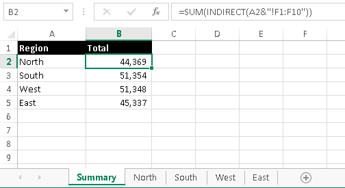
Figure 50-2:
Using the INDIRECT function to create references.
This formula concatenates the text in A2 with a range reference. The INDIRECT function evaluates the result and converts it to an actual range reference. The result is equivalent to this formula:
=SUM(North!F1:F10)
This formula is copied down the column. Each formula returns the sum of range F1:F10 on the corresponding worksheet.
Making a cell reference unchangeable
Another use for the INDIRECT function is to create a reference to a cell that never changes. For example, consider this formula, which sums the values in the first 12 rows of column A:
=SUM(A1:A12)
If you insert a new row 1, Excel changes the formula to
=SUM(A2:A13)
In other words, the formula adjusts so that it continues to refer to the original data (and it no longer sums the first 12 rows of column A). To prevent Excel from changing the cell references, use the INDIRECT function:
=SUM(INDIRECT(“A1:A12”))
This formula
always
returns the sum of the first 12 rows in column A.
Tip 51: Formula Editing in Dialog Boxes
This is a simple tip, but one that most users don’t know about.
When Excel displays a dialog box that accepts a range reference, the field that contains the range reference is always in
point
mode. For example, consider the New Name dialog box, shown in Figure 51-1. This dialog box appears when you choose Formulas⇒Defined Names⇒Define Name.
If you activate the Refers to Field and use the arrow keys to edit the range reference, you’ll find that you’re actually pointing to a range in the worksheet — not editing the reference text. The solution: Press F2.
The F2 key toggles between point mode and edit mode. In edit mode, the arrow keys work the same as when you’re editing a formula. Also notice that the current mode is displayed in the left corner of the status bar.
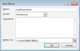
Figure 51-1:
The Refers To field defaults to point mode. Press F2 to switch to edit mode.
This tip applies to all Excel dialog boxes that contain range selection fields.
Tip 52: Converting a Vertical Range to a Table
Often, tabular data is imported into Excel as a single column. Figure 52-1 shows an example. Column A contains employee information, and each “record” consists of three consecutive cells in a single column: Name, Department, and Location. The goal is to convert this data so that each record appears in a single row, with three columns.
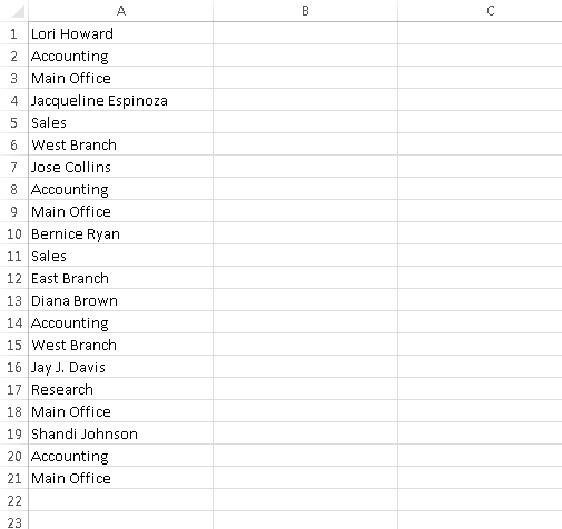
Figure 52-1:
Vertical data that needs to be converted to three columns.
You can convert this type of data several ways, but here’s a method that’s fairly easy. It uses a single formula, which is copied to a range.
Enter the following formula in cell C1, and then copy it down and across.
=INDIRECT(“A” &COLUMN()-2 + (ROW()-1)*3)
Figure 52-2 shows the transformed data in C1:E7.
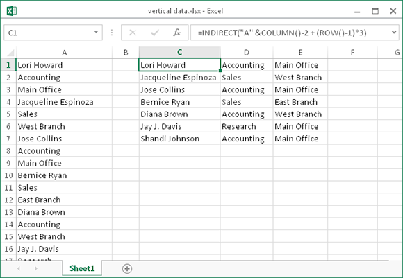
Figure 52-2:
Vertical data transformed to a table.
The formula works for vertical data that uses three cells per record, but it can be modified to handle vertical data that uses any number of cells per record by changing the “3” in the formula. For example, if the vertical data has five fields, use this formula:
=INDIRECT(“A” &COLUMN()-2 + (ROW()-1)*5)
Part IV: Working with Data
In this part, you’ll find tips related to working with data of all types. There’s an excellent chance that the tips here will improve your overall efficiency.
Tips and Where to Find Them
Tip 53:
Selecting Cells Efficiently
Tip 54:
Automatically Filling a Range with a Series
Tip 55:
Fixing Trailing Minus Signs
Tip 56:
Restricting Cursor Movement to Input Cells
Tip 57:
Transforming Data with and Without Using Formulas
Tip 58:
Creating a Drop-Down List in a Cell
Tip 59:
Comparing Two Ranges by Using Conditional Formatting
Tip 60:
Finding Duplicates by Using Conditional Formatting
Tip 61:
Working with Credit Card Numbers
Tip 62:
Identifying Excess Spaces
Tip 64:
Using Flash Fill to Extract Data
Tip 65:
Using Flash Fill to Combine Data
Tip 66:
Inserting Stock Information
Tip 67:
Getting Data from a Web Page
Tip 68:
Importing a Text File into a Worksheet Range
Tip 69:
Using the Quick Analysis Feature
Tip 70:
Filling the Gaps in a Report
Tip 71:
Performing Inexact Searches
Tip 53: Selecting Cells Efficiently
Many Excel users think that the only way to select a range of cells is to drag over the cells with the mouse. Although selecting cells with a mouse works, it’s rarely the most
efficient
way to accomplish the task. A better way is to use your keyboard to select ranges.
Selecting a range by using the Shift and arrow keys
The simplest way to select a range is to press (and hold) Shift and then use the arrow keys to highlight the cells. For larger selections, you can use PgDn or PgUp while pressing Shift to move in larger increments.
You can also use the End key to quickly extend a selection to the last non-empty cell in a row or column. To select the range B3:B8 (see Figure 53-1) by using the keyboard, move the cell pointer to B3 and then press the Shift key while you press End followed by the down-arrow key. Similarly, to select B3:D3, press the Shift key while you press End, followed by the right-arrow key.
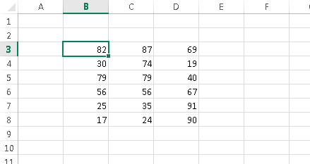
Figure 53-1:
A range of cells.
Selecting the current region
Often, you need to select a large rectangular selection of cells — the
current region
. To select the entire block of cells, move the cell pointer anywhere within the range and press Ctrl+A.
 If the cell pointer is within a table (created by using Insert⇒Tables⇒Table), pressing Ctrl+A selects only the data. Press Ctrl+A a second time to select the table’s Header row and Total row.
Selecting a range by Shift+clicking
When you’re selecting a very large range, using the mouse may be the most efficient method — but dragging is not required. Select the upper-left cell in the range. Then scroll to the lower-right corner of the range, press Shift, and click the lower-right cell.
Selecting noncontiguous ranges
Most of the time, your range selections are probably simple rectangular ranges. In some cases, you may need to make a
multiple selection
— a selection that includes nonadjacent cells or ranges. For example, you may want to apply formatting to cells in different areas of your worksheet. If you make a multiple selection, you can apply the formatting in one step to all selected ranges. Figure 53-2 shows an example of a multiple selection.
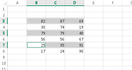
Figure 53-2:
A multiple selection that consists of noncontiguous ranges.
You can select a noncontiguous range by using either the mouse or the keyboard.
Press Ctrl as you click and drag the mouse to highlight individual cells or ranges.
From the keyboard, select a range as described previously (by using the Shift key). Then press Shift+F8 to select another range without canceling the previous range selection. Repeat this action as many times as needed. When you’re finished, press Shift+F8 again to return to normal selecting mode.
Selecting entire rows
To select a single row, click a row number along the left of the worksheet. Or select any cell in the row and press Shift+spacebar.
To select multiple adjacent rows, click and drag in the row number area. Or select any cell in the first (or last) row and press Shift+spacebar to select the row. Then press Shift and use the arrow keys to extend the row selection down (or up).
To select multiple nonadjacent rows, press Ctrl while you click the row numbers for the rows you want to include.
Selecting entire columns
To select a single column, click a column letter along the top of the worksheet. Or select any cell in the column and press Ctrl+spacebar.
To select multiple adjacent columns, click and drag in the column letter section. Or select any cell in the first (or last) column and press Ctrl+spacebar to select the column. Then press Shift and use the arrow keys to extend the selection to the right (or left).
To select multiple nonadjacent columns, press Ctrl while you click the column letters for the columns you want to include.
Selecting multisheet ranges
In addition to two-dimensional ranges on a single worksheet, ranges can extend across multiple worksheets to be three-dimensional ranges.
Figure 53-3 shows a simple example of a multisheet workbook. The workbook has four sheets, named Totals, Operations, Marketing, and Manufacturing. The sheets are laid out identically.
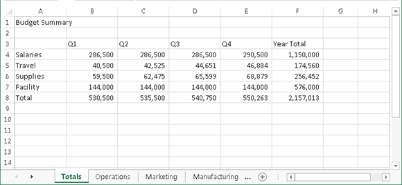
Figure 53-3:
Each worksheet in this workbook is laid out identically.
Assume that you want to apply the same formatting to all sheets — for example, you want to make the column headings bold with background shading. Selecting a multisheet range is the best approach. When the ranges are selected, the formatting is applied to all sheets.
In general, selecting a multisheet range is a simple two-step process:
1.
Select the range in one sheet.
2.
Select the worksheets to include in the range.
 To select a group of contiguous worksheets, press Shift and click the sheet tab of the last worksheet that you want to include in the selection. To select individual worksheets, press Ctrl and click the sheet tab of each worksheet that you want to select. When you make the selection, the sheet tabs of the selected sheets appear with a white background, and Excel displays [Group] on the title bar. When you finish working with the multisheet range, click any sheet tab to leave Group mode.
Tip 54: Automatically Filling a Range with a Series
If you need to fill a range with a series of values, one approach is to enter the first value, write a formula to calculate the next value, and copy the formula. For example, Figure 54-1 shows a series of consecutive numbers in column A. Cell A1 contains the value 1, and cell A2 contains this formula, which was copied down the column:
=A1+1
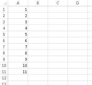
Figure 54-1:
Excel offers an easy way to generate a series of values like these.
Another approach is to let Excel do the work by using the handy AutoFill feature:
1.
Enter 1 into cell A1.
2.
Enter
2
into cell A2.
3.
Select A1:A2.
4.
Move the mouse cursor to the lower-right corner of cell A2 (the cell’s
fill handle
), and when the mouse pointer turns into a black plus sign, drag down the column to fill in the cells.
 You can turn this behavior on and off. If cells don’t have a fill handle, choose File⇒Options and click the Advanced tab in the Excel Options dialog box. Select the check box labeled Enable Fill Handle and Cell Drag-And-Drop.
The data entered in Steps 1 and 2 provide Excel with the information it needs to determine which type of series to use. If you entered 3 in cell A2, the series will consist of odd integers: 1, 3, 5, 7, and so on.
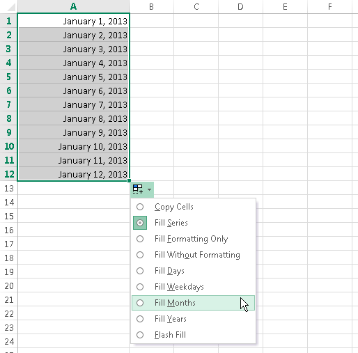
When you release the mouse button after dragging, Excel displays an Auto Fill Options drop-down list. Click to select other options. The list of options is particular helpful with dates. Figure 54-2 shows the Auto Fill Options when working with a date series. You can quickly create a series of weekdays, months, or years.
