Authors: Mehmed Kantardzic
Data Mining (118 page)

we can see that middle parts of the strings were really exchanged as in a standard crossover operation. On the other hand, the two new strings remain as valid permutations since the symbols are actually permuted within each string.
The other steps of a GA applied to the TSP are unchanged. A GA based on the above operator outperforms a random search for TSP, but still leaves much room for improvement. Typical results from the algorithm, when applied to 100 randomly generated cities gave after 20,000 generations, a value of the whole tour 9.4% above minimum.
13.6 MACHINE LEARNING USING GAs
Optimization problems are one of the most common application categories of GAs. In general, an optimization problem attempts to determine a solution that, for example, maximizes the profit in an organization or minimizes the cost of production by determining values for selected features of the production process. Another typical area where GAs are applied is the discovery of input-to-output mapping for a given, usually complex, system, which is the type of problem that all machine-learning algorithms are trying to solve.
The basic idea of input-to-output mapping is to come up with an appropriate form of a function or a model, which is typically simpler than the mapping given originally—usually represented through a set of input–output samples. We believe that a function best describes this mapping. Measures of the term “best” depend on the specific application. Common measures are accuracy of the function, its robustness, and its computational efficiency. Generally, determining a function that satisfies all these criteria is not necessarily an easy task; therefore, a GA determines a “good” function, which can then be used successfully in applications such as pattern classification, control, and prediction. The process of mapping may be automated, and this automation, using GA technology, represents another approach to the formation of a model for inductive machine learning.
In the previous chapters of this book we described different algorithms for machine learning. Developing a new model (input-to-output abstract relation) based on some given set of samples is an idea that can also be implemented in the domain of GAs. There are several approaches to GA-based learning. We will explain the principles of the technique that is based on schemata and the possibilities of its application to classification problems.
Let us consider a simple database, which will be used as an example throughout this section. Suppose that the training or learning data set is described with a set of attributes where each attribute has its categorical range: a set of possible values. These attributes are given in Table
13.4
.
TABLE 13.4.
Attributes A
i
with Possible Values for a Given Data Set s
| Attributes | Values |
| A 1 | x, y, z |
| A 2 | x, y, z |
| A 3 | y, n |
| A 4 | m, n, p |
| A 5 | r, s, t, u |
| A 6 | y, n |
The description of a classification model with two classes of samples, C1 and C2, can be represented in an
if-then
form where on the left side is a Boolean expression of the input features’ values and on the right side its corresponding class:


These classification rules or classifiers can be represented in a more general way: as some strings over a given alphabet. For our data set with six inputs and one output, each classifier has the form
where p
i
denotes the value of the
i
th attribute (1 ≤ i ≤ 6) for the domains described in Table
13.4
, and d is one of two classes. To describe the classification rules in a given form, it is necessary to include the “don’t care” symbol “*” into the set of values for each attribute. For example, the new set of values for attribute A
1
is {x, y, z, *}. Similar extensions are given for other attributes. The rules that were given earlier for classes C
1
and C
2
can be decomposed to the segments under conjunction (AND logical operation) and expressed as


To simplify the example, we assume that the system has to classify into only two classes: C
1
and
not
C
1
. Any system can be easily generalized to handle multiple classes (multiple classification). For a simple classification with a single rule C
1
we can accept only two values for d: d = 1 (member of the class C
1
) and d = 0 (not a member of the class C
1
).
Let us assume that at some stage of the learning process, there is a small and randomly generated population of classifiers Q in the system, where each classifier is given with its strength s:
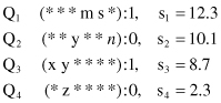
Strengths s
i
are parameters that are computed based on the available training data set. They show the fitness of a rule to the training data set, and they are proportional to the percentage of the data set supported by the rule.
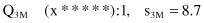
The basic iterative steps of a GA, including corresponding operators, are applied here to optimize the set of rules with respect to the fitness function of the rules to training data set. The operators used in this learning technique are, again, mutation and crossover. However, some modifications are necessary for mutation. Let us consider the first attribute A
1
with its domain {x, y, z, *}. Thus, when mutation is called, we would change the mutated character (code) to one of the other three values that have equal probability. The strength of the offspring is usually the same as that of its parents. For example, if mutation is the rule Q
3
on the randomly selected position 2, replacing the value y with a randomly selected value *, the new mutated classifier will be