Authors: Mehmed Kantardzic
Data Mining (85 page)

Suppose data samples are given with n attributes (A
1
, A
2
, … , A
n
). Attributes can be categorical or continuous. For a continuous attribute, we assume that its values are discretized into intervals in the preprocessing phase. A training data set T is a set of samples such that for each sample there exists a class label associated with it. Let C = {c
1
, c
2
, … , c
m
} be a finite set of
class labels
.
In general, a pattern P = {a
1
, a
2
, … , a
k
} is a set of attribute values for different attributes (1 ≤ k ≤ n). A sample is said to match the pattern P if it has all the attribute values given in the pattern. For rule R: P → c, the number of data samples matching pattern P and having class label c is called the
support
of rule R, denoted
sup(R)
. The ratio of the number of samples matching pattern P and having class label c versus the total number of samples matching pattern P is called the
confidence
of R, denoted as
conf(R)
. The association-classification method (CMAR) consists of two phases:
1.
rule generation or training, and
2.
classification or testing.
In the first, rule generation phase, CMAR computes the complete set of rules in the form R: P → c, such that sup(R) and conf(R) pass the given thresholds. For a given support threshold and confidence threshold, the associative-classification method finds the complete set of class-association rules (CAR) passing the thresholds. In the testing phase, when a new (unclassified) sample comes, the classifier, represented by a set of association rules, selects the rule that matches the sample and has the highest confidence, and uses it to predict the classification of the new sample.
We will illustrate the basic steps of the algorithm through one simple example. Suppose that for a given training data set T, as shown in Table
10.3
, the support threshold is 2 and the confidence threshold is 70%.
TABLE 10.3.
Training Database T for the CMAR Algorithm
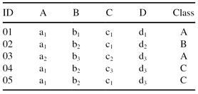
First, CMAR scans the training data set and finds the set of attribute values occurring beyond the threshold support (at least twice in our database). One simple approach is to sort each attribute and to find all frequent values. For our database T, this is a set F = {a
1
, b
2
, c
1
, d
3
}, and it is called a frequent itemset. All other attribute values fail the support threshold. Then, CMAR sorts attribute values in F, in support-descending order, that is, F-list = (a
1
, b
2
, c
1
, d
3
).
Now, CMAR scans the training data set again to construct an FP tree. The FP tree is a prefix tree with respect to the F-list. For each sample in a training data set, attributes values appearing in the F-list are extracted and sorted according to the order in the F-list. For example, for the first sample in database T, (a
1
, c
1
) are extracted and inserted in the tree as the left-most branch in the tree. The class label of the sample and the corresponding counter are attached to the last node in the path.
Samples in the training data set share prefixes. For example, the second sample carries attribute values (a
1
, b
2
, c
1
) in the F-list and shares a common prefix a
1
with the first sample. An additional branch from the node a
1
will be inserted in the tree with new nodes b
2
and c
1
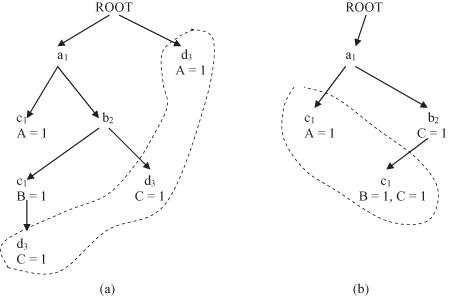
. A new class label B with the count equal to 1 is also inserted at the end of the new path. The final FP tree for the database T is given in Figure
10.7
a.
Figure 10.7.
FP tree for the database in Table
10.3
. (a) nonmerged FT tree; (b) FT tree after merging d
3
nodes.
After analyzing all the samples and constructing an FP tree, the set of CAR can be generated by dividing all rules into subsets without overlap. In our example it will be four subsets: (1) the rules having d
3
value; (2) the rules having c
1
but no d
3
; (3) the rules having b
2
but neither d
3
nor c
1
; and (4) the rules having only a
1
. CMAR finds these subsets one by one.
To find the subset of rules having d
3
, CMAR traverses nodes having the attribute value d
3
and looks “upward” the FP tree to collect d
3
-projected samples. In our example, there are three samples represented in the FP tree, and they are (a
1
, b
2
, c
1
, d
3
):C, (a
1
, b
2
, d
3
):C, and (d
3
):A. The problem of finding all FPs in the training set can be reduced to mining FPs in the d
3
-projected database. In our example, in the d
3
-projected database, since the pattern (a
1
, b
2
, d
3
) occurs twice its support is equal to the required threshold value 2. Also, the rule based on this FP, (a
1
, b
2
, d
3
) → C has a confidence of 100% (above the threshold value), and that is the only rule generated in the given projection of the database.
After a search for rules having d
3
value, all the nodes of d
3
and their corresponding class labels are merged into their parent nodes at the FP tree. The FP tree is shrunk as shown in Figure
10.7
b. The remaining set of rules can be mined similarly by repeating the previous procedures for a c
1
-projected database, then for the b
2
-projected database, and finally for the a
1
-projected database. In this analysis, (a
1
, c
1
) is an FP with support 3, but all rules are with confidence less than the threshold value. The same conclusions can be drawn for pattern (a
1
, b
2
) and for (a
1
). Therefore, the only association rule generated through the training process with the database T is (a
1
, b
2
, d
3
) → C with support equal to 2 and 100% confidence.
When a set of rules is selected for classification, CMAR is ready to classify new samples. For the new sample, CMAR collects the subset of rules matching the sample from the total set of rules. Trivially, if all the rules have the same class, CMAR simply assigns that label to the new sample. If the rules are not consistent in the class label, CMAR divides the rules into groups according to the class label and yields the label of the “strongest” group. To compare the strength of groups, it is necessary to measure the “combined effect” of each group. Intuitively, if the rules in a group are highly positively correlated and have good support, the group should have a strong effect. CMAR uses the strongest rule in the group as its representative, that is, the rule with highest χ
2
test value (adopted for this algorithm for a simplified computation). Preliminary experiments have shown that CMAR outperforms the C4.5 algorithm in terms of average accuracy, efficiency, and scalability.
10.7 MULTIDIMENSIONAL ASSOCIATION–RULES MINING
A multidimensional transactional database DB has the schema
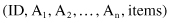
where ID is a unique identification of each transaction, A
i
are structured attributes in the database, and items are sets of items connected with the given transaction. The information in each tuple t = (id, a
1
, a
2
, … , a
n
, items-t) can be partitioned into two: dimensional part (a
1
, a
2
, … , a
n
) and itemset part (items-t). It is commonsense to divide the mining process into two steps: first mine patterns about dimensional information and then find frequent itemsets from the projected sub-database, or vice versa. Without any preferences in the methodology we will illustrate the first approach using the multidimensional database DB in Table
10.4
.
TABLE 10.4.
Multidimensional-Transactional Database DB
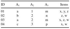
One can first find the frequent multidimensional-value combinations and then find the corresponding frequent itemsets of a database. Suppose that the threshold value for our database DB in Table
10.4
is set to 2. Then, the combination of attribute values that occurs two or more than two times is frequent, and it is called a multidimensional pattern or MD pattern. For mining MD patterns, a modified Bottom Up Computation (BUC) algorithm can be used (it is an efficient “iceberg cube” computing algorithm). The basic steps of the BUC algorithm are as follows:
1.
First, sort all tuples in the database in alphabetical order of values in the first dimension (A
1
), because the values for A
1
are categorical. The only MD pattern found for this dimension is (a, *, *) because only the value
a
occurs two times; the other values b and c occur only once and they are not part of the MD patterns. Value * for the other two dimensions shows that they are not relevant in this first step, and they could have any combination of allowed values.
Select tuples in a database with found M pattern (or patterns). In our database, these are the samples with ID values 01 and 03. Sort the reduced database again with respect to the second dimension (A
2
), where the values are 1 and 2. Since no pattern occurs twice, there are no MD patterns for exact A
1
and A
2
values. Therefore, one can ignore the second dimension A
2
(this dimension does not reduce the database further). All selected tuples are used in the next phase.
Selected tuples in the database are sorted in alphabetical order of values for the third dimension (in our example A
3
with categorical values). A subgroup (a, *, m) is contained in two tuples and it is an MD pattern. Since there are no more dimensions in our example, the search continues with the second step.
2.
Repeat the processes in step 1; only start not with the first but with the second dimension (first dimension is not analyzed at all in this iteration). In the following iterations, reduce the search process further for one additional dimension at the beginning. Continue with other dimensions.