More Guns Less Crime (39 page)
Read More Guns Less Crime Online
Authors: John R. Lott Jr
Tags: #gun control; second amendment; guns; crime; violence

An effective as well as moving piece I recently read was written by Dale Anema, a father whose son was trapped for hours inside the Columbine High School building during the April 1999 attack. His agony while waiting to hear what happened to his son touches any parent's worst fears. Because he had witnessed this tragedy, he described his disbelief over the policy debate:
Two pending gun bills are immediately dropped by the Colorado legislature. One is a proposal to make it easier for law-abiding citizens to carry concealed weapons; the other is a measure to prohibit municipalities from suing gun manufacturers. I wonder: If two crazy hoodlums can walk into a "gun-free" zone full of our kids, and police are totally incapable of defending the children, why would anyone want to make it harder for law-abiding adults to defend themselves and others? ... Of course, nobody on TV mentions that perhaps gun-free zones are potential magnets to crazed killers. 140
Qppgndhr One
How to Account for the Different Factors That Affect Crime and How to Evaluate the Importance of the Results
The research in this book relies on what is known as regression analysis, a statistical technique that essentially lets us "fit a line" to a data set. Take a two-variable case involving arrest rates and crime rates. One could simply plot the data and draw the line somewhere in the middle, so that the deviations from the line would be small, but each person would probably draw the line a little differently. Regression analysis is largely a set of conventions for determining exactly how the line should be drawn. In the simplest and most common approach—ordinary least squares (OLS)—the line chosen minimizes the sum of the squared differences between the observations and the regression line. Where the relationship between only two variables is being examined, regression analysis is not much more sophisticated than determining the correlation.
The regression coefficients tell us the relationship between the two variables. The diagram in figure Al.l indicates that increasing arrest rates decreases crime rates, and the slope of the line tells us how much crime rates will fall if we increase arrest rates by a certain amount. For example, in terms of figure Al, if the regression coefficient were equal to — 1, lowering the arrest rate by one percentage point would produce a similar percentage-point increase in the crime rate. Obviously, many factors account for how crime changes over time. To deal with these, we use what is called multiple regression analysis. In such an analysis, as the name suggests, many explanatory (or exogenous) variables are used to explain how the endogenous (or dependent) variable moves. This allows us to determine whether a relationship exits between different variables after other effects have already been taken into consideration. Instead of merely drawing a line that best fits a two-dimensional plot of data points, as shown in figure Al.l, multiple regression analysis fits the best line through an
246 / APPENDIX ONE 100%
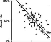
©VBest-fit" line
0% 50% 100%
Crime rate
Figure A 1.1. Fitting a regression line to a scatter diagram
n-dimensional data plot, where n is the number of variables being examined.
A more complicated regression technique is called two-stage least squares. We use this technique when two variables are both dependent on each other and we want to try to separate the influence of one variable from the influence of the other. In our case, this arises because crime rates influence whether the nondiscretionary concealed-handgun laws are adopted at the same time as the laws affect crime rates. Similar issues arise with arrest rates. Not only are crime rates influenced by arrest rates, but since an arrest rate is the number of arrests divided by the number of crimes, the reverse also holds true. As is evident from its name, the method of two-stage least squares is similar to the method of ordinary least squares in how it determines the line of best fit—by minimizing the sum of the squared differences from that line. Mathematically, however, the calculations are more complicated, and the computer has to go through the estimation in two stages.
The following is an awkward phrase used for presenting regression results: "a one-standard-deviation change in an explanatory variable explains a certain percentage of a one-standard-deviation change in the various crime rates." This is a typical way of evaluating the importance of statistical results. In the text I have adopted a less stilted, though less precise formulation: for example, "variations in the probability of arrest account for 3 to 11 percent of the variation in the various crime rates." As I will explain below, standard deviations are a measure of how much variation a given variable displays. While it is possible to say that a one-percentage-point change in an explanatory variable will affect the crime rate by a certain amount (and, for simplicity, many tables use such phrasing whenever possible), this approach has its limitations. The reason is
APPENDIX ONE/247
that a 1 percent change in the explanatory variable may sometimes be very unlikely: some variables may typically change by only a fraction of a percent, so assuming a one-percentage-point change would imply a much larger impact than could possibly be accounted for by that factor. Likewise, if the typical change in an explanatory variable is much greater than 1 percent, assuming a one-percentage-point change would make its impact appear too small.
The convention described above—that is, measuring the percent of a one-standard-deviation change in the endogenous variable explained by a one-standard-deviation change in the explanatory variable—solves the problem by essentially normalizing both variables so that they are in the same units. Standard deviations are a way of measuring the typical change that occurs in a variable. For example, for symmetric distributions, 68 percent of the data is within one standard deviation of either side of the mean, and 95 percent of the data is within two standard deviations of the mean. Thus, by comparing a one-standard-deviation change in both variables, we are comparing equal percentages of the typical changes in both variables. 1
The regressions in this book are also "weighted by the population" in the counties or states being studied. This is necessitated by the very high level of "noise" in a particular year's measure of crime rates for low-population areas. A county with only one thousand people may go through many years with no murders, but when even one murder occurs, the murder rate (the number of murders divided by the county's population) is extremely high. Presumably, no one would believe that this small county has suddenly become as dangerous as New York City. More populous areas experience much more stable crime rates over time. Because of this difficulty in consistently measuring the risk of murder in low-population counties, we do not want to put as much emphasis on any one year's observed murder rate, and this is exactly what weighting the regressions by county population does.
Several other general concerns may be anticipated in setting up the regression specification. What happens if concealed-handgun laws just happen to be adopted at the same time that there is a downward national trend in crime rates? The solution is to use separate variables for the different years in the sample: one variable equals 1 for all observations during 1978 and zero for all other times, another equals 1 for all observations during 1979 and zero otherwise, and so on. These "year-dummy" variables thus capture the change in crime from one year to another that can only be attributed to time itself. Thus if the murder rate declines nationally from 1991 to 1992, the year-dummy variables will measure the average decline in murder rates between those two years and allow us to
ask if there was an additional drop, even after accounting for this national decline, in states that adopted nondiscretionary concealed-handgun laws.
A similar set of "dummy" variables is used for each county in the United States, and they measure deviations in the average crime rate across counties. Thus we avoid the possibility that our findings may show that nondiscretionary concealed-handgun laws appear to reduce crime rates simply because the counties with these laws happened to have low crime rates to begin with. Instead, our findings should show whether there is an additional drop in crime rates after the adoption of these laws.
The only way to properly account for these year and county effects, as well as the influences on crime from factors like arrest rates, poverty, and demographic changes, is to use a multiple-regression framework that allows us to directly control for these influences.
Unless we specifically state otherwise, the regressions reported in the tables attempt to explain the natural logarithms of the crime rates for the different categories of crime. Converting into "logs" is a conventional method of rescaling a variable so that a given absolute numerical change represents a given percentage change. (The familiar Richter scale for measuring earthquakes is an example of a base-10 logarithmic scale, where a tremor that registers 8 on the scale is ten times as powerful as one that registers 7, and one that registers 7 is ten times as powerful as one that registers 6.) The reason for using logarithms of the endogenous variable rather than their simple values is twofold. First, using logs avoids giving undue importance to a few, very large, "outlying" observations. Second, the regression coefficient can easily be interpreted as the percent change in the endogenous variable for every one-point change in the particular explanatory variable examined.
Finally, there is the issue of statistical significance. When we estimate coefficients in a regression, they take on some value, positive or negative. Even if we were to take two completely unrelated variables—say, sun-spot activity and the number of gun permits—a regression would almost certainly yield a coefficient estimate other than zero. However, we cannot conclude that any positive or negative regression coefficient really implies a true relationship between the variables. We must have some measure of how certain the coefficient estimate is. The size of the coefficient does not really help here—even a large coefficient could have been generated by chance.
This is where statistical significance enters in. The measure of statistical significance is the conventional way of reporting how certain we can be that the impact is different from zero. If we say that the reported number is "positive and statistically significant at the 5 percent level," we mean that there is only a 5 percent chance that the coefficient happened to
APPENDIX ONE/249
take on a positive value when the true relationship in fact was zero or negative. 2 To say that a number is statistically significant at the 1 percent level represents even greater certainty. The convention among many social scientists is usually not to affirm conclusions unless the level of significance reaches 10 percent or lower; thus, someone who says that a result is "not significant" most likely means that the level of significance failed to be as low as 10 percent.
These simple conventions are, however, fairly arbitrary, and it would be wrong to think that we learn nothing from a value that is significant at "only" the 11 percent level, while attaching a great deal of weight to one that is significant at the 10 percent level. The true connection between the significance level and what we learn involves a much more continuous relationship. We are more certain of a result when it is significant at the 10 percent level rather than at the 15 percent level, and we are more certain of a result at the 1 percent level than at the 5 percent level.
Appendix Two
Explanations of Frequently Used Terms
Arrest rate: The number of arrests per crime.
Crime rate: The number of crimes per 100,000 people.
Cross-sectional data: Data that provide information across geographic areas (cities, counties, or states) within a single period of time.
Discretionary concealed-handgun law: Also known as a "may-issue" law; the term discretionary means that whether a person is ultimately allowed to obtain a concealed-handgun permit is up to the discretion of either the sheriff or judge who has the authority to grant the permit. The person applying for the permit must frequently show a "need" to carry the gun, though many rural jurisdictions automatically grant these requests.
Endogenous: A variable is endogenous when changes in the variable are assumed to caused by changes in other variables.
Exogenous: A variable is exogenous when its values are as given, and no attempt is made to explain how that variable's values change over time.
Externality: The costs of or benefits from one's actions may accrue to other people. External benefits occur when people cannot capture the beneficial effects that their actions produce. External costs arise when people are not made to bear the costs that their actions impose on others.
Nondiscretionary concealed-handgun law: Also known as a "shall-issue" or "do-issue" law; the term nondiscretionary means that once a person meets certain well-specified criteria for obtaining a concealed-handgun permit, no discretion is involved in granting the permit—it must be issued.