Simply Complexity (10 page)
Authors: Neil Johnson

(1) Real-world Complex Systems contain collections of objects whose complicated overall interactions feature feedback and
memory. By contrast, our intern problem featured a single systematic intern who relentlessly applied the same complicated mathematical rule over and over again.
(2) In order to produce the wide variety of outputs such as Chaos and fractals, the systematic intern had to manually change the value of
r
. In other words, the intern becomes the “invisible hand” or central controller that is absent from real-world Complex Systems. Instead, real-world Complex Systems can move around between order and disorder of their own accord.
(3) It is inconceivable that any living object – such as a driver or trader, animal or even a living cell – can go through its entire existence taking actions which are dictated by a single, highly-complicated mathematical rule such as the one presented earlier. The complexity observed in real-world systems cannot have been generated simply by applying such a rule over and over again.
Later in the book we will focus on real-world systems in which points (1) and (2) are important. Here we look more closely at point (3). As we all know, real people are not as systematic as our systematic-intern example claimed they could be. In fact they probably have moments when they are systematic and moments when they are not. I know I do – and I know quite a few others that do as well. After all, we are only human. We know from section 3.2 that a completely careless intern will produce a time-series that is random. So what happens if we have a more realistic intern – one who is neither completely systematic nor completely careless? We need to know this, since when we deal with Complex Systems involving a collection of people, there will undoubtedly be such a mix of both things going on. Not only will there be some people behaving more systematically than others at any one moment, but these people’s behavior will itself change over time. This is the case that we now consider – the more realistic intern – and this will nicely bridge the gap between completely systematic but complicated behavior such as Chaos, and completely random behavior. In particular, the output time-series will lie between complete order and complete randomness. Not only that, but the type of patterns produced will turn out to be mirrored in a wide range of human activities – from music and art through to human conflict and financial market trading. Moreover these are also the
types of patterns that are observed in physical systems as diverse as the sizes and shapes of galaxies through to the coastlines of countries. The upshot is that there is indeed a type of
universal pattern of Life
lying somewhere in the middle-ground between completely ordered patterns and completely disordered patterns. And such patterns are produced by objects that are neither completely systematic nor completely random – in other words, objects like us. So it looks like we really do live in some kind of middle-ground.
So what happens in our filing problem with one file and many shelves, where the intern isn’t completely systematic but also isn’t completely careless? Since anything not completely systematic will have, by definition, an element of carelessness, our analysis will involve coins being flipped to mimic this carelessness effect. We will keep thinking about one file and many shelves – but instead of letting the intern move the file from any one shelf to any other, we will for simplicity restrict him to moving the file by at most one shelf, either upward or downward. This is perfectly fine for illustrating what we want to illustrate, and could easily be generalized. It also mirrors a lot of real-world systems where the changes from one step to another are reasonably gradual.
Here is our modified story. Each day, our intern will shift the file up or down one shelf – and we will look at what happens as we move from this being done in a completely random way, through to it being done in a systematic way. Let us start off with the completely random way – in other words, we have a careless intern. And the fact that this careless intern is equally likely to move the file up or down one shelf is equivalent to saying that he moves the file according to the toss of a coin. So each day, the intern tosses a coin: if it is heads, he moves the file up one shelf; if it is tails, he moves it down one shelf. Since there are many shelves, and we can assume that the file starts off somewhere near the middle, we won’t need to worry about the file reaching the top or bottom. So, if the file starts on shelf 10, for example, the time-series showing its location over consecutive days might look as follows:
10 11 10 9 10 11 12 11 12 13 . . .
In technical jargon, the file is undergoing a
random walk
or a
drunkard’s walk
since a drunkard presumably has equal chances of walking forward or backward at each step, like the file. The coin-toss rule that our careless intern applies doesn’t have any memory. In other words, the coin is equally likely to show heads or tails on a given day irrespective of the previous outcomes. Coins don’t remember anything – and nor, supposedly, do drunkards.
But that may be unfair on drunkards. What happens if the drunkard
does
remember what general direction he is heading in? In other words he has some memory of the past. In the filing context, this corresponds to making the intern more systematic. We can simulate this effect of adding memory, and hence adding feedback to the coin-toss operation, by saying that the likelihood of tossing heads depends on what has happened in the past. Using the technical jargon we have come across earlier in this book, we are gradually adding memory or
feedback
to the dynamics. And what we will find is that this feedback – which we have already stated is a crucial ingredient of Complex Systems – helps create exactly the same kinds of patterns which are observed in the output time-series of many real-world Complex Systems.
The memory, or feedback, that we will add is simple. If the file happens to be moving upward, for example, it will then have an increased chance of continuing to move upward. Likewise if the file happens to be moving downward, it will have an increased chance of continuing to move downward. This is equivalent to saying that the coin is biased in such a way that the random walk now has some memory in it. An example of the resulting time-series showing the location of the file, would be:
10 11 12 11 12 13 14 13 14 15 . . .
Since the earlier time-series without any memory was called a drunkard’s walk, we could call this a “slightly sober drunkard’s walk” if we wanted. Now if we continue making this slightly sober drunkard’s walk increasingly sober – and hence increasingly biased – then eventually the file would move as follows:
10 11 12 13 14 15 16 17 18 19 . . .
and this is exactly the output time-series that a systematic intern would produce if he was moving the file up one shelf every step. It is also the outcome we would get from a completely sober walker walking steadily down the street.
So the random-walk of the file gradually becomes less random, and ends up as a steady walk. But how can we characterize this a bit more scientifically? This opens up one of the hard questions that scientists have – they can often see some kind of order, but need to find a way of characterizing it. Now, each time the intern carries out the experiment with a given bias in the coins, he will get a slightly different answer. Therefore whatever way we find of characterizing the order will need to be a statistical way. In other words, it tells us what is happening on average. More specifically, it is the result of averaging over lots of different experiments with the same setup – so, lots of different offices or lots of different drunkards with the same memory.
It turns out that the way in which scientists typically characterize such walks, relates to the drunkenness of the person doing the walking. Consider the sober walker, who walked as you and I would typically walk down a street. Recall that the position at successive steps is given by:
10 11 12 13 14 15 16 17 18 19 . . .
In other words, after nine steps he has moved a distance equal to nine, i.e. since the final position is 19 and the initial position was 10, he has moved a distance 19–10 = 9 in 9 steps. Equivalently, the file moves 19–10 = 9 shelves in nine steps. This means that the distance moved is nine, in a time interval of nine steps. The distance moved can therefore be written as
t
a
where
a
= 1 and
t
= 9. (Any number calculated to the power of one is equal to the number itself. Just try it on a calculator.) Note that we could have also referred to the sober walker as creating a perfectly persistent walk, since he always persists in the same direction as he is already going. By contrast, recall the output time-series for the completely drunk walker, or equivalently the file position when being moved by the completely careless intern:
10 11 10 9 10 11 12 11 12 13 . . .
In this case, after nine steps he has moved a distance equal to about three, i.e. since the final position is 13 and the initial position was 10, he has moved a distance 13–10 = 3 in 9 steps. Now, we know that 3 × 3 = 9, or equivalently that three is the square root of nine. In mathematical terms, this can be written as 3 = √9 or equivalently 3 = 9
0.5
. This means that the approximate distance moved can be written as
t
a
where
a
= 0.5, as opposed to
a
= 1 for the sober walker. In other words, the approximate distance moved can be written as 9
0.5
, as opposed to 9
1
for the sober walker.
For intermediate cases where the walker is neither completely sober nor completely drunk – or, equivalently, where the intern is neither completely systematic nor completely careless – the approximate distance moved can be written as
t
a
where
a
is larger than 0.5 but smaller than 1. Just look at the output time-series that we had earlier for this case:
10 11 12 11 12 13 14 13 14 15 . . .
The distance moved in
t
= 9 timesteps is 15–10 = 5, which can be written as
t
a
with
a
given approximately by 0.74.
So as we span the range from drunk to sober, the corresponding walk goes from covering an approximate distance of
t
a
with
a
= 0.5, to
t
a
with
a
= 1. Equivalently, if we span the range from a careless intern to a systematic intern, the change in file position goes from an approximate distance of
t
a
with
a
= 0.5, to
t
a
with
a
= 1. In other words, the walk increases in its persistence. By contrast, now imagine we had biased the walk such that there was an anti-persistence in terms of carrying on in one direction. This could be achieved by biasing the coin-tossing so that an outcome of heads would more likely be followed by an outcome of tails. In this case, the approximate distance moved would be given by
t
a
with
a
less than 0.5 but greater than
a
= 0. An extreme case would be where the bias was such that every heads is followed by a tails and vice versa – hence every move up by one shelf is followed by a move down by one shelf and vice versa. In this case, the distance moved after nine steps will be just one. Using
t
a
then gives
a
= 0 since any number calculated to the power of zero is equal to one.
We have therefore found a way of characterizing the order, or conversely the disorder, in an output time-series by calculating the approximate distance moved, and then relating this to the number of timesteps using
t
a
.
This procedure then gives a particular value of
a.
For technical reasons, some scientists prefer to think about a number
D
defined by
a
=
1/D.
So
a
= 0.5 corresponds to
D
= 2, since 0.5 = 1/2, and
a
= 1 corresponds to
D
= 1, since 1 = 1/1. Furthermore, since this is a statistical characterization of how ordered the output time-series is, we could refer to the resulting number
D
(or equivalently 1/a) as a statistical dimension. This means that for a value of
a
between
a
= 0.5 and
a
= 1, the dimension is between
D
= 2 and
D
= 1. And as we saw earlier, since any number between 1 and 2 is a fraction, we could legitimately refer to this as a fractional dimension. In other words, an output time-series with a fractional value of
D,
is a fractal.
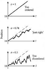
To refer to such a walk as a fractal, makes sense when we think about the shape of the resulting output time-series.
Figure 3.3
shows sketches of typical shapes for the cases which we have
discussed:
a
= 0.5,
a
= 0.74 and
a
= 1. Of all the shapes shown, the one that looks closest to that observed, say, in real mountain ranges or coastlines, is the one with
a
= 0.74. In other words it is neither too jagged, nor too smooth. By contrast, the others look too jagged, such as
a
= 0.5, or too smooth, such as
a
= 1. Another way of saying the same thing is that the output time-series for
a
= 0.5 and hence
D
= 2, is too disordered (or too random) for a real mountain range or coastline. On the other hand, the output time-series for
a
= 1 and hence
D
= 1, can be said to look too ordered (or too systematic, or too deterministic).