Read The Amazing Story of Quantum Mechanics Online
Authors: James Kakalios
The Amazing Story of Quantum Mechanics (13 page)

BOOK: The Amazing Story of Quantum Mechanics
12.22Mb size Format: txt, pdf, ePub
ads
There is one aspect of Heisenberg’s theory that has generated way too much blather and misinformation to be ignored—that is, the famed uncertainty principle. If you’ll bear with me, I’d like to take a brief detour to set the record straight about what the uncertainty principle does and does not mean. It’s actually not too complicated, that is, once one accepts that there is a wavelike nature to matter.
The uncertainty principle posits a relationship between the uncertainty of the location of a particle and the uncertainty of its momentum. Heisenberg saw that the product of these two uncertainties must be bigger than a constant that turns out to be (wait for it) Planck’s constant,
h,
divided by 4 times π. Why Planck’s constant is divided by 4π has to do with technical aspects of waves that need not concern us here. The fact that
h
turns up again and again when describing the atomic regime indicates that Planck’s initial guess about the graininess of energy was on target, and by introducing
h
he discovered a new fundamental constant of nature, as important for understanding how the universe is put together as the value of the speed of light or the charge of an electron.
Right off the bat let me emphasize that the uncertainty principle does
not
restrict the precision with which I can measure the position of a particle, nor that of its momentum. Neither does it state that one can never measure the position and momentum of a particle simultaneously, but it does get to the heart of what such a measurement entails.
not
restrict the precision with which I can measure the position of a particle, nor that of its momentum. Neither does it state that one can never measure the position and momentum of a particle simultaneously, but it does get to the heart of what such a measurement entails.
Suppose that I can experimentally determine the position of an electron and at the same time the momentum of this electron (I’ll describe how in a moment). I may find that the electron is at a location x = 2.34528976543901765438 cm as reckoned from a given point, and the momentum has a value of p = 14.254489765539989021 kg-meter/sec. There are certainly a large number of decimal places in these measurements, but in order to convince myself that this is indeed the electron’s position and momentum, I repeat the experiment, under exactly the same conditions. If those are in fact the true values of position and momentum, I should be able to reproduce
all
of those decimal places. Performing the experiment a second time, I now find that the electron’s position is x = 2.3452891120987693790 cm and the momentum is p = 14.2544100876495832002 kg-meter/ sec. On the one hand, the first few digits in both the x and p measurements agree exactly with what was found before, but on the other hand after a few decimal places the overlap with the first observation disappears.
What I find, after repeating the experiment many more times, is that the
average
position of the electron is 2.32428 cm and the
average
momentum is 14.254 kg-meter/sec, as illustrated in Figure 16. That is, the only measurements that one really can trust are of the average position and momentum. I can make a plot of the num-ber of times a particular value of the position is observed against the value of the position. Such a plot would look, after a large number of trials, like the familiar bell-shaped curve, known and feared by students throughout recorded history. The peak in the curve would represent the value of the position that was observed most frequently and would also indicate the average location of the electron. At the highest point, the curve is very narrow. Halfway down the curve, there is a width that is referred to as the “standard deviation.” The standard deviation is an indication of how much we can trust the average value resulting from this bell-shaped curve. The bigger the standard deviation, the greater the possible uncertainty in the average value. It is these standard deviations, also referred to in mathematics as uncertainties, that are constrained by the Heisenberg uncertainty principle.
average
position of the electron is 2.32428 cm and the
average
momentum is 14.254 kg-meter/sec, as illustrated in Figure 16. That is, the only measurements that one really can trust are of the average position and momentum. I can make a plot of the num-ber of times a particular value of the position is observed against the value of the position. Such a plot would look, after a large number of trials, like the familiar bell-shaped curve, known and feared by students throughout recorded history. The peak in the curve would represent the value of the position that was observed most frequently and would also indicate the average location of the electron. At the highest point, the curve is very narrow. Halfway down the curve, there is a width that is referred to as the “standard deviation.” The standard deviation is an indication of how much we can trust the average value resulting from this bell-shaped curve. The bigger the standard deviation, the greater the possible uncertainty in the average value. It is these standard deviations, also referred to in mathematics as uncertainties, that are constrained by the Heisenberg uncertainty principle.

Figure 16:
Plot of the histogram of measured positions (a) and momenta (b). The vertical dashed lines represent the average values of position and momentum, and the small arrows indicate the standard deviation for each measurement.
Plot of the histogram of measured positions (a) and momenta (b). The vertical dashed lines represent the average values of position and momentum, and the small arrows indicate the standard deviation for each measurement.
As an illustration of standard deviations, consider a class of 100 students taking a final exam. If all 100 students receive exactly the same score of 50 points out of 100, then the average grade will be 50 and the standard deviation will be 0. That is, if you are told that the average grade is 50 with a standard deviation of 0, then there is no ambiguity or uncertainty in what any given student scored on the exam. Now, if 90 students receive a score of 50 points, while 5 students score a 55 and the remaining 5 receive a grade of 45, the average grade would remain 50, but now there is a small width to the distribution of grades. While the average value is still 50, some students have a score that differs from the average value. There is now some small but non-zero question as to whether a student chosen at random will have a grade equal to the average score of 50 or not. In an extreme case, all 100 students in the class could receive different grades, from as low as 1 or 2, through 48, 49, 50, and 51, up to 98, 99, and 100. The average grade would
still
be 50,
27
but now the distribution would range from 1 through 100. Only 1 student out of 100 would have an actual grade on the final exam that is exactly equal to the average score of the class, and the large size of the standard deviation would indicate that the average grade was not a particularly meaningful or insightful indicator of any given student’s performance. When dealing with large numbers, the two questions one must ask are: What is the average? and What is the standard deviation?
Returning to my simultaneous measurements of an electron’s position and momentum, I found that after repeated trials there was a bell-shaped curve for the position, which gave its average location, and another bell-shaped curve for the momentum. It is the standard deviations of these two bell-shaped curves that the Heisenberg uncertainty principle addresses. Heisenberg’s theory tells us that the standard deviation of the electron’s position is connected to the standard deviation of the electron’s momentum, so that changes in one affect the other. The widths of the two distributions in Figure 16 are not independent, and efforts to narrow one will necessarily broaden the other. Heisenberg calculated that the product of the two standard deviations cannot be smaller than
h
/4π. Any experiment that manages to decrease the standard deviation of the momentum (for example) will necessarily broaden the standard deviation of the position.
h
/4π. Any experiment that manages to decrease the standard deviation of the momentum (for example) will necessarily broaden the standard deviation of the position.
Why would the standard deviation of an electron’s position be related to the standard deviation of its momentum? Because of the de Broglie wave associated with the motion of the electron. The wavelength of this matter-wave is in a sense a measure of how precisely we can say where the electron is, and this wavelength is connected to the electron’s momentum by the relation (momentum) × (wavelength) =
h.
h.
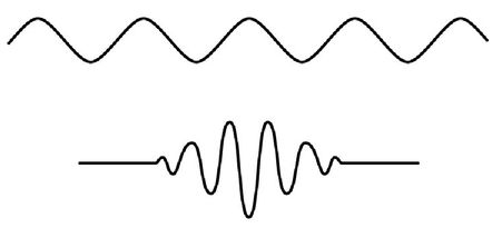
Figure 17:
Sketch of two possible de Broglie matter waves for an electron. In the top curve, the electron is associated with a single wave. As one needs only one wavelength to describe the wave, the momentum is perfectly known, but at the cost of an infinite uncertainty in the location of the electron. In the bottom curve many different waves, each with different wavelengths, have been added to yield a “wavepacket.” The uncertainty in the spatial location of the electron is reduced, but there is a corresponding increase in uncertainty in the electron’s momentum.
Sketch of two possible de Broglie matter waves for an electron. In the top curve, the electron is associated with a single wave. As one needs only one wavelength to describe the wave, the momentum is perfectly known, but at the cost of an infinite uncertainty in the location of the electron. In the bottom curve many different waves, each with different wavelengths, have been added to yield a “wavepacket.” The uncertainty in the spatial location of the electron is reduced, but there is a corresponding increase in uncertainty in the electron’s momentum.
Assume that the electron’s momentum is precisely known, with absolutely no ambiguity. Then the average momentum
is
the momentum, just as in our classroom example when all 100 students received the same grade on the final of 50. There is one value for the wavelength of the matter-wave for this perfectly known momentum, as shown in the top cartoon in Figure 17. A pure wave by definition extends forever, from one end of the universe to the other. Where would we say the location of the electron would be for such a perfect wave? Its average value might be well defined, but its standard deviations would be infinitely large.
The Heisenberg connection between the standard deviations of the position and momentum results from the fact that the location of the electron is connected to the wavelength of the matter-wave, which in turn is related to the object’s momentum. In order to shrink the standard deviation of the electron’s position, the electron’s matter-wave should be zero except for a small region near the average position. But in order to construct a wave packet such as this, illustrated by the lower sketch in Figure 17, one needs to add many waves together, all of slightly different wavelengths, so that they would destructively cancel out beyond a narrow region around the average position. Since the wavelength is connected to the momentum through (momentum) × (wavelength) =
h,
adding many different wavelengths together is the same as saying that there is a broad range of momentum values for the localized electron. The tighter the limits with which we wish to specify the electron’s location, that is, the smaller the position’s standard deviation, the more different wavelengths we have to combine and the greater the corresponding standard deviation of the momentum. The two standard deviations are thus joined together, through the matter-wave relation (momentum) × (wavelength) =
h.
Of course, we can measure an electron’s position to any arbitrary precision we wish—as long as we do not care about its momentum, and vice versa. Whether the electron has a well-defined momentum (with no standard deviation) or a well-defined position (also with no standard deviation) depends on what measurement I perform. There can be no answer until the question is posed, and how I ask the question determines what answer I’ll obtain.
The bundle of waves described above, and shown in the lower sketch in Figure 17, is technically referred to as a “wave packet.” It makes no sense to ask where the electron is located, on a scale smaller than the extent of the wave packet. How do I measure the momentum of an electron? One way would be to record its position at two different times. Knowing how far it moved, and how long it took to travel this distance, I can determine its velocity, and multiplying by the mass (assuming I can avoid relativistic corrections) yields the momentum. How can I tell where the electron is at the two different times? It’s easy to tell the velocity of an automobile—you just look at where it is at two different times. How do I look at an electron? The same way I look at a car—by shining light on it and having the light be reflected to my eye (or some other detector). Cars are much larger than the wavelength of visible light, but to observe the electron I need light with a wavelength smaller than the extent of the electron’s wave packet. The connection between wavelength and frequency for light is given by the simple relationship (frequency) × (wavelength) = speed of light. Since the speed of light is a constant, the smaller the wavelength, the larger the frequency of the light, and from energy = h × (frequency), the larger the energy of the light photon. Thus, to measure the momentum of an electron with a very small wave packet (small uncertainty in position), I must strike it with a very high-energy photon. When the photon reflects from the electron, the electron’s recoil changes its momentum. When a careful mathematical analysis is performed, one finds that you cannot do better than the Heisenberg uncertainty principle. You may think there might be a clever scheme to get around this limitation of the wavelength of light to determine the electron’s position and momentum—but many have tried and all have failed.
We might have been spared countless inane pronouncements that “quantum mechanics has proven that everything is uncertain” if Heisenberg had simply named his principle something a little
less
catchy, such as “the principle of complementary standard deviations.”
less
catchy, such as “the principle of complementary standard deviations.”
Armed now with an appreciation for the physical content of the famous uncertainty principle, we now consider the following classic example of nerd humor:
Werner Heisenberg is pulled over for speeding by a highway patrolman. The police officer walks over to Werner’s car, leans over, and asks Heisenberg, “Do you know how fast you were going?”
Heisenberg replies, “No, but I know where I am!”
BOOK: The Amazing Story of Quantum Mechanics
12.22Mb size Format: txt, pdf, ePub
ads
Other books
King's Test by Margaret Weis
Hanging by a Moment (From this Moment Book 1) by Walker, Eva
Business as Usual by Hughes, E.
Health And Wholeness Through The Holy Communion by Prince, Joseph
A Sentimental Traitor by Dobbs, Michael
Buzzkill (Pecan Bayou Series) by Trent, Teresa
Drowning Lessons by Peter Selgin
Renounced by Bailey Bradford
On China by Henry Kissinger
The Sword and the Sorcerer by Norman Winski