Collected Essays (37 page)

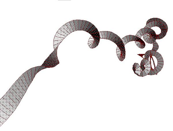
Stretching a Slinky turns curvature into torsion.

Here’s a little algebra problem: Given the formulae for kappa and tau in terms of R and H, and given that R
²
+ H
²
= A
²
, what can you say about the sum kappa
²
+ tau
²
? The answer tells you more about the nature of a Slinky’s trade-off between curvature and torsion.

One fact that seems odd at first is that the curvature and torsion of a helix are dependent on the size of the helix. If you make both R and H five times as big, you make the torsion and curvature 1/10 as big. If you make R and H N times as big, you make the curvature and torsion 1/(2*N) as big.

But this makes sense if you think of a fly that switches from a small helix to a big helix; the fly is indeed changing the way that it’s flying, so it makes sense that the kappa and the tau should change.

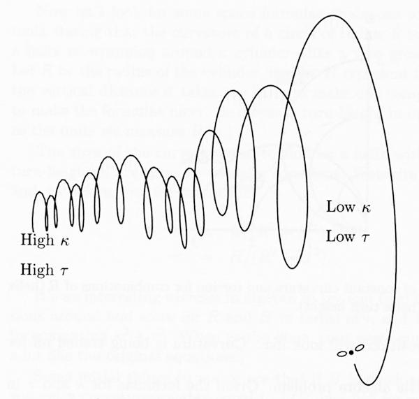
Changing Curvature and Torsion.

This observation suggests a simple way to express the difference between flies and birds—flies fly with much higher curvature and torsion than do the birds. Gnats, for that matter, fly even more tightly knotted paths, and have very large values of curvature and torsion.

Just as in the plane, a space curve can be specified in terms of natural equations that give the curvature and torsion as functions of the arclength. These equations have the form kappa = f(s) and tau = g(s). The shape and size of the space curve is uniquely determined by the curvature and the torsion functions. The next two figures show two intriguing space curves given by simple curvature and torsion functions.

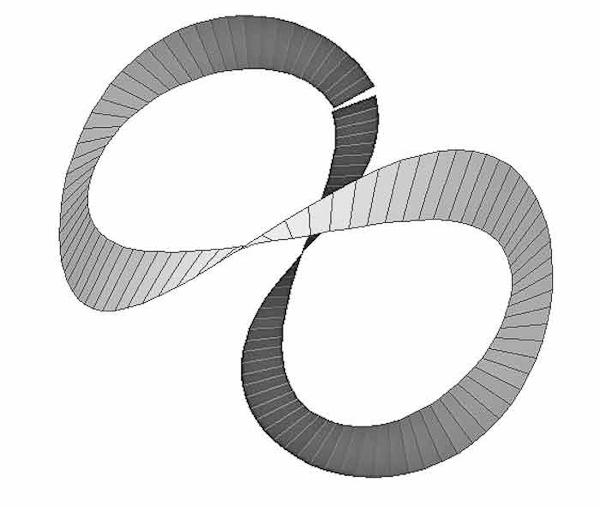
The “baseball stitch curve,” more properly called the “rocker,” with natural equations kappa = 1 and tau = sine(arclength).

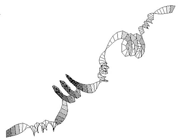
The phone-cord, with natural equations kappa = 10*sine(arclength) and tau = 3.

Note that the phone cord is a space curve where we do allow ourselves to put in negative values for the curvature.

There is not a large literature on these “kappatau” curves, so I’ve given my own names to these two: the rocker, and the phone-cord.

At one time I thought that the rocker was a correct way to represent the seam on a tennis-ball or the stitching on a baseball, but an email from the mathematician John Horton Conway convinced me I was wrong. Conway makes the anthropological conjecture that every time a mathematician discovers a curve that he or she thinks might be the true baseball curve, the curve is a different one!

An analysis of the
real-world
baseball stitch curve can be found in a web-published paper: Richard Thompson, “Designing A Baseball Cover,” you can search it out online. It turns out the baseball stitch curve is based on something so prosaic as a patented 1860s pen and ink drawing of a plane shape used to cut out the leather for a half of a baseball, a shape arrived at by trial and error. Thompson finds a fairly gnarly closed-form approximation of this shape.

Not only does my rocker fail to match the baseball stitch curve, it can be proved that the rocker curve does not in fact lie on the surface of a sphere. My thanks to Roger Alpert for unearthing the following fact: the rocker fails to satisfy the following necessary condition for lying on the surface of the sphere, where s stands for arclength (see Yung-Chow Wong, “On An Explicit Characterization of Spherical Curves,” Proceedings of the American Mathematical Society 34 (July, 1972) pp. 239-242.).

d/ds[(1/tau)*d/ds(1/kappa)] + tau*(1/kappa) = 0

(For kappa = 1 and tau = sin(s), the left-hand side of this is sin(s), which isn’t identically 0.)

Numerical estimates indicate that the arclength of the rocker has exactly twice the length of a circle of the same radius. This suggests an easy way to make a rocker. Cut out two identical annuli (thick circles) from some fairly stiff paper (manila file folders are good), cut radial slits in the annuli, tape two of the slit-edges together, bend the annuli in two different ways (one like a clockwise helix and one like a counterclockwise helix) and tape the other two slit-edges together, forming a continuous band of double length . Because an annulus cannot bend along its osculating plane, the curvature of the shape is fixed along the arclength. Because half the band is like a clockwise helix and half is like a counterclockwise helix, when the shape relaxes, the torsion presumably varies with the arclength like a sine wave function that goes between plus one and minus one. The torsion seems to be zero at the two places where the slits are taped together. Note that I have not
proved
that my empirical paper rocker is the same as my mathematical rocker, this is simply my conjecture.

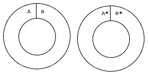
Make your own rocker.

How to make your own rocker curve:

Make a larger copy of the figure above on stiff paper.

Cut along all solid lines.

Tape edge A to edge B* with the letters on the same side.

Bend the two rings in the opposite sense.

Tape edge A* to edge B with the letters on the same side.

How were the computerized images of the rocker and the phone cord generated? They use an algorithm based on the 1851 formulae of Serret and Frenet (see, for instance, Dirk Struik,
Lectures on Classical Differential Geometry
, Addison-Wesley, Reading, Mass, 1961.). Let’s state the formulae in “differential” form. The question the formulae address is this: when we do a small displacement ds along a space curve, what is the displacement dT, dN, and dB of the vectors in the moving trihedron?

dT =(kappa*N)*ds

dN =(-kappa*T + tau*B)*ds

dB =(- tau*N)*ds

The first and third equations correspond, respectively, to the definitions of curvature and torsion. The second equation describes the “back-reaction” of the T and B motions on N.

[A mathematician’s way to remember the Frenet formulae is to note that if we think of the ds multipliers on the right-hand sides of the three equations as linear combinations of T, N, and B, then the coefficients in these combinations make a three-by-three antisymmetric matrix, that is, a matrix in which the ji entry is the negative of the ij entry.]

Since we are lucky enough to live in three-dimensional space, it’s possible for us to experiment with our bodies and to perceive directly why the Serret-Frenet formulae are true. To experience the equations, you should, if possible, stick out your right hand’s thumb, index finger, and middle finger as shown earlier. Now start trying to “fly” your trihedron around according to these rules:

(1) The index finger always points in the direction your hand is moving. (2) You are allowed to turn the index finger towards or away from direction of the middle finger by a motion corresponding to rotating around the axis of your thumb. (3) You are allowed to turn the thumb towards or away from the middle finger by a motion corresponding to rotating around the axis of your forefinger.

To get clear on what’s meant by motion (2), grab your thumb with you left hand and make as if you were trying to unscrew it from your hand. This is a kind of “yawing” motion, and it corresponds to the first of the three Serret-Frenet formulae: the change in the tangent is equal to the curvature times normal. Motion (3) corresponds to grabbing your index finger with your left hand and trying to unscrew that finger. This is a kind of “rolling” motion, and it corresponds to the third of the Serret-Frenet formulae: the change in the binormal is the negative of the torsion times the normal.

In thinking of flying along a space curve you should explicitly resist thinking about boats and airplanes which have a built-in visual trihedron which generally does not correspond to the moving trihedron of the space curve. If you do want to think about a machine, imagine a rocket which never slows down and never speeds up, which can turn left or right—relative to you the passenger—and which can roll. Or better yet, think about being a cybernetic house-fly.

An exciting thing about the Frenet-Serret formulae is that they lend themselves quite directly to creating a numerical computer simulation to create kappatau space curves with arbitrary curvature and torsion. To write the code in readable form, we can “overload” the arithmetic operators to do the expected things to our vector objects. A scalar times a vector changes the length of the vector, while a vector times a vector invokes the vector cross product. In addition we add a vector function called Normalize such that if a vector A invokes the method by calling A.Normalize(), then A becomes a unit vector. Here is the heart of an algorithm for updating the position P of a point on an arbitrary kappatau curve.

P = P + ds * T;

s = s + ds;

T = T + (kappa(s) * ds) * N;

B = B + ( -tau(s) * ds) * N;

T.Normalize();

B.Normalize();

N = (B * T);

As far as I know, very little mathematical work has been done with kappatau curves because in the past nobody could visualize them. I first implemented the algorithm as a so-called notebook for the Mathematica software, and then I wrote a stand-alone Windows program called Kaptau. You can my Mathematica notebooks or the stand-alone Windows program from my web-site.

So how do I think flies fly? I think that they generally move along at a constant speed like a space curve parameterized by its arclength, and that they manage to loiter here and speed away from there by varying their curvature and torsion between low and high values. As mathematicians like to say (even when they’re wrong): “It’s obvious!”