Collected Essays (36 page)
Authors: Rudy Rucker

Curvature along circular arcs in the plane.
We often represent a curve in the plane by an equation involving x and y coordinates. Most calculus students remember a brief, nasty encounter with Newton’s formula for the curvature of a curve; the formula uses fractional powers and the first and second derivatives of y with respect to x. Fortunately, there is no necessity for us to trundle out this cruel, ancient idol. Instead we think of curvature as a primitive notion and express the curve in a more natural way.
The idea is that instead of talking about positions relative to an arbitrary x axis and y axis, we think of a curve as being a bent number-line by itself. The curve is marked off in units of “arclength”, where arclength is the distance measured along the curve, just as if the curve were a piece of rope that you could stretch out next to a ruler. We’ll use the variable s to stand for arclength and the infinitesimal ds to stand for a very small bit of arclength. If we think of a curve in x and y coordinates, we can define ds as the square root of dx squared plus dy squared, and we can then use integration to add up the ds quantities to get a value for s. But in this essay, we’ll instead think of s an ds as primitive quantities.
If we think of the arclength s as primitive, the most natural way to describe a plane curve is by an equation that gives the curvature directly as a function of arclength, an equation of the form k = f(s), where the Greek letter k or kappa is the commonly used symbol for curvature. The next figure shows two famous plane curves which happen to have simple expressions for curvature as a function of arclength. The catenary curve is the shape assumed by a chain (or bridge cable) suspended from two points, while the logarithmic spiral is a form very popular among our friends the mollusks.
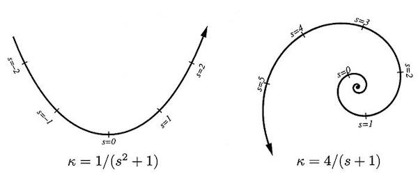
The catenary and the logarithmic spiral expressed by natural equations, with curvature k being a function of arclength s. Arclength is marked as units along the curves.
Note that for the spiral, the center is where s approaches -1. And if you jump over the anomalous central point and push down into larger negative values of s, you produce a mirror-image of the spiral.
It would be nice to also think of space curves in a natural, coordinate-free way—surely this is the way a fly buzzing around in the center of an empty room must think. Profound mathematical insights come hard, and it was a hundred and twenty years after Clairaut before the correct way to represent a space curve by intrinsic natural equations was finally discovered—by the French mathematicians Joseph Alfred Serret and Frederic-Jean Frenet.
The idea is that at each point of a space curve one can define two numerical quantities called curvature and torsion. The curvature of a space curve is essentially the same as the curvature k of a plane curve: it measures how rapidly the curve is bending to one side. The torsion measures a curve’s tendency to twist out of a plane. We use the Greek letter t or tau to stand for torsion. But what exactly is meant by “bend to one side,” and “twist out of a plane”? Which plane?
The idea is that at each point P of a space curve you can define three mutually perpendicular unit-length vectors: the tangent T, the normal N, and the binormal B. T shows the direction the curve is moving in, N lies along the direction which the curve is currently bending in, and B is a vector perpendicular to T and N. (In terms of the vector cross product, T cross N is B, N cross B is T, and B cross T is N.) For space curves we ordinarily work only with positive values of curvature, and have N point in the direction in which the curve is actually bending. (In certain of the analytical curves we’ll look at later we relax this condition and allow negative curvature of space curves.)
Taken together, T, N and B make up the so-called “moving trihedron of a space curve”. In the figure below, we show part of a space curve (actually a helix) with several instances of the moving trihedron. So that it’s easier to see the three-dimensionality of the image, we draw the curve as a ribbon like a twisted ladder. The curve runs along one edge of the ladder, and the rungs of the ladder correspond to the directions of successive normals to the curve.
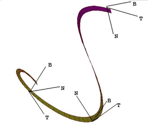
The moving trihedron of a space curve: T the tangent, N the normal, and B the binormal.
To understand exactly how the normal is defined, it helps to think of the notion of the “osculating” (kissing) plane. At each point of a space curve there is some plane that best fits the curve at that point. The tangent vector T lies in this plane, and the direction perpendicular to T in this plane holds the normal N. The binormal is a vector perpendicular to the osculating plane.
With the idea of the moving trihedron in mind, we can now say that the curvature measures the rate at which the tangent turns, and the torsion measures the rate at which the binormal turns.
Note that T, N and B are always selected so as to form a right-handed coordinate system. This means that if you hold out the thumb, index finger and middle finger of your right hand, these directions correspond to the tangent, the normal, and the binormal.
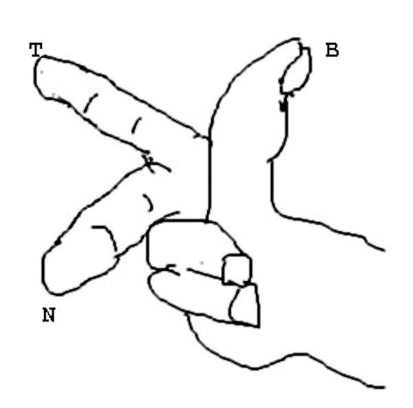
A right-hand as a trihedron.
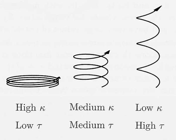
Just as the circle is the plane curve characterized by having constant curvature, the helix is the space curve characterized by having constant curvature and constant torsion. Figure 5 shows how the signs of the curvature and torsion affect the shapes of plane and space curves.
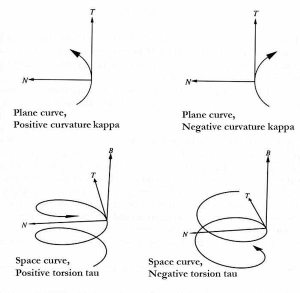
How the signs of the curvature and torsion affect the motion of a curve.
Now let’s look for some space formulae analogous to the plane formula stating that the curvature of a circle of radius R is 1/R. Think of a helix as wrapping around a cylinder—like a vine growing up a post. Let R be the radius of the cylinder, and let H represent the turn-height: the vertical distance it takes the helix to make one complete turn (and to make the formulae nicer, we measure turn-height in units 2*pi as large as the units we measure R in.)
The sizes of the curvature and torsion on a helix with radius R and turn-height H are given by two nice equations. We write “tau” for torsion and, as before, “kappa” for curvature:
kappa = R / (R
2
+ H
2
), and
tau = H / (R
2
+ H
2
).
It’s an interesting exercise in algebra to try and turn these two equations around and solve for R and H in terms of kappa and tau. (Hint: Start by computing kappa
2
+ tau
2
. When you’re done, your new equations will look a lot like the original equations.)
Some initial things to notice are that if H is much smaller than R, you get a curvature roughly equal to 1/R, just like for a circle, and a tau very close to 0. If, on the other hand, R is very close to zero, then the torsion is roughly 1/H while the curvature is close to 0. A fly which does a barrel-roll while moving through a nearly straight distance of H has a torsion of 1/H. The faster it can roll, the greater is its torsion.
A less obvious fact is that if we look down on a plane showing all possible positive combinations R and H, the lines of constant curvature lie on semi-circles with their two endpoints on the R-axis; while the points representing constant torsion lie on semi-circles with their two endpoints on the H-axis. The curvature and torsion combinations gotten by stretching a given Slinky lie along a quarter circle centered on the origin. Apparently the two families of semi-circles are perpendicular to each other.
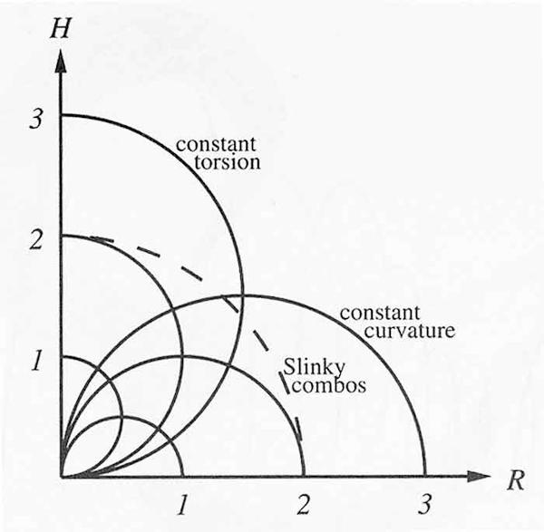
Lines of constant curvature and torsion for combinations of R (helix radius) and H (helix turn height).
Suppose I have a helix like a steel Slinky spring. What happens to the curvature and the torsion as I stretch a single turn of it without untwisting? Suppose that the initial radius of the helix is A. Given the physical fact that the length of one twist of the Slinky keeps the same length, you can show that as you stretch it, R
2
+ H
2
will stay constant at a value of A
2
, which corresponds to a circle of radius A around the origin of the R-H plane. As you stretch a Slinky loop with the particular starting radius of 2, its R and H values will move along the dotted blue line shown in Figure 6. Figure 7 shows what a few of the intermediate positions will look like. Curvature is being traded off for torsion.