Statistics Essentials For Dummies (13 page)

Chapter 5
:
The Normal Distribution
In This Chapter
Understanding the normal and standard normal distributions
Going from start to finish with regular normal probabilities
Working backward to find percentiles
There are two major types of random variables: discrete and continuous.
Discrete
random variables basically count things (number of heads on 10 coin flips, number of female Democrats in a sample, and so on). The most well known discrete random variable is the binomial (see Chapter 4). A
continuous
random variable measures things and takes on values within an interval, or they have so many possible values that they might as well be deemed continuous (for example, time to complete a task, exam scores, and so on).
In this chapter, you work on finding probabilities for the most famous continuous random variable, the normal. You also find percentiles for the normal distribution (where you are given a probability as a percent) and you have to find the value of
X
that's associated with it.
Basics of the Normal Distribution
We say that
X
has a normal distribution if its values fall into a smooth (continuous) curve with a bell-shaped, symmetric pattern, meaning it looks the same on each side when cut down the middle. The total area under the curve is 1. Each normal distribution has its own mean,, and its own standard deviation,
. For intro stat courses, the mean and standard deviation for the normal distribution are given to you.
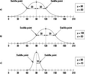
Figure 5-1 illustrates three different normal distributions with different means and standard deviations.
Figure 5-1:
Three normal distributions.
Note that the
saddle points
(highlighted by arrows in Figure 5-1 on either side of the mean) on each graph are where the graph changes from concave down to concave up. The distance from the mean out to either saddle point is equal to the standard deviation for the normal distribution. For any normal distribution, almost all its values lie within three standard deviations of the mean.
The Standard Normal (Z) Distribution
One very special member of the normal distribution family is called the standard normal distribution, or
Z
-distribution. The
Z-distribution
is used to help find probabilities and solve other types of problems when working with any normal distribution.
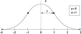
The standard normal (
Z
) distribution has a mean of zero and a standard deviation of 1; its graph is shown in Figure 5-2. A value on the
Z
-distribution represents the number of standard deviations the data is above or below the mean; these are called
z
-scores or
z
-values. For example,
z
= 1 on the
Z
-distribution represents a value that is 1 standard deviation above the mean. Similarly,
z
= -1 represents a value that is one standard deviation below the mean (indicated by the minus sign on the
z
-value).
Figure 5-2:
The
Z
-distribution has a mean of 0 and standard deviation of 1.
Because probabilities for any normal distribution are nearly impossible to calculate by hand, we use tables to find them. All the basic results you need to find probabilities for any normal distribution can be boiled down into one table based on the standard normal (
Z
) distribution. This table is called the
Z
-table and is found in the appendix as Table A-1. All you need is one formula to transform your normal distribution (
X
) to the standard normal (
Z
) distribution, and you can use the
Z
-table to find the probability you need.
The general formula for changing a value of
X
into a value of
Z
is. You take your
x
-value, subtract the mean, and
divide by the standard deviation; this gives you its corresponding
z
-value.
For example, if
X
is a normal distribution with mean 16 and standard deviation 4, the value 20 on the
X
-distribution would transform into 20 - 16 divided by 4, which equals 1. So, the value 20 on the
X
-distribution corresponds to the value 1 on the
Z
-distribution. Now use the
Z
-table to find probabilities for
Z
, which are equivalent to the corresponding probabilities for
X
. Table A-1 (appendix) shows the probability that
Z
is less than any value between -3 and +3.

