Read Structure and Interpretation of Computer Programs Online
Authors: Harold Abelson and Gerald Jay Sussman with Julie Sussman
Structure and Interpretation of Computer Programs (49 page)

In figure
3.5
we see the environment structure created
by evaluating the expression
(f 5)
. The call to
f
creates
a new environment E1 beginning with a frame in which
a
, the
formal parameter of
f
, is bound to the argument 5. In E1, we
evaluate the body of
f
:
(sum-of-squares (+ a 1) (* a 2))
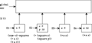 |
To evaluate this combination, we first evaluate the subexpressions.
The first subexpression,
sum-of-squares
, has a value that is a
procedure object. (Notice how this value is found: We first look in
the first frame of E1, which contains no binding for
sum-of-squares
. Then we proceed to the enclosing environment,
i.e. the global environment, and find the binding shown in
figure
3.4
.) The other two subexpressions are
evaluated by applying the primitive operations
+
and
*
to
evaluate the two combinations
(+ a 1)
and
(* a 2)
to
obtain 6 and 10, respectively.
Now we apply the procedure object
sum-of-squares
to the
arguments 6 and 10. This results in a new environment E2 in which the
formal parameters
x
and
y
are bound to the arguments.
Within E2 we evaluate the combination
(+ (square x) (square y))
.
This leads us to evaluate
(square x)
, where
square
is
found in the global frame and
x
is 6. Once again, we set up a
new environment, E3, in which
x
is bound to 6, and within this
we evaluate the body of
square
, which is
(* x x)
. Also as
part of applying
sum-of-squares
, we must evaluate the
subexpression
(square y)
, where
y
is 10. This second call
to
square
creates another environment, E4, in which
x
, the
formal parameter of
square
, is bound to 10. And within E4 we
must evaluate
(* x x)
.
The important point to observe is that each call to
square
creates a new environment containing a binding for
x
. We can
see here how the different frames serve to keep separate the different
local variables all named
x
. Notice that each frame created by
square
points to the global environment, since this is the
environment indicated by the
square
procedure object.
After the subexpressions are evaluated, the results are
returned. The values generated by the two calls to
square
are
added by
sum-of-squares
, and this result is returned by
f
.
Since our focus here is on the environment structures, we will not
dwell on how these returned values are passed from call to call;
however, this is also an important aspect of the evaluation process,
and we will return to it in detail in chapter 5.
Exercise 3.9.
In section
1.2.1
we used the substitution model to analyze two
procedures for computing factorials, a recursive version
(define (factorial n)
(if (= n 1)
1
(* n (factorial (- n 1)))))
and an iterative version
(define (factorial n)
(fact-iter 1 1 n))
(define (fact-iter product counter max-count)
(if (> counter max-count)
product
(fact-iter (* counter product)
(+ counter 1)
max-count)))
Show the environment structures created by evaluating
(factorial 6)
using each version of the
factorial
procedure.
14
We can turn to the environment model to see how procedures and
assignment can be used to represent objects with local state. As an
example, consider the “withdrawal processor” from
section
3.1.1
created by calling the
procedure
(define (make-withdraw balance)
(lambda (amount)
(if (>= balance amount)
(begin (set! balance (- balance amount))
balance)
"Insufficient funds")))
Let us describe the evaluation of
(define W1 (make-withdraw 100))
followed by
(W1 50)
50
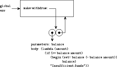
Figure
3.6
shows the result of defining the
make-withdraw
procedure in the global environment. This produces a
procedure object that contains a pointer to the global environment.
So far, this is no different from the examples we have already seen,
except that the body of the procedure is itself a
lambda
expression.
 |
The interesting part of the computation happens when we apply the
procedure
make-withdraw
to an argument:
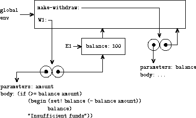
(define W1 (make-withdraw 100))
We begin, as usual, by setting up an environment E1 in which the
formal parameter
balance
is bound to the argument 100. Within
this environment, we evaluate the body of
make-withdraw
, namely
the
lambda
expression. This constructs a new procedure object,
whose code is as specified by the
lambda
and whose environment
is E1, the environment in which the
lambda
was evaluated to
produce the procedure. The resulting procedure object is the value
returned by the call to
make-withdraw
. This is bound to
W1
in the global environment, since the
define
itself is being
evaluated in the global environment. Figure
3.7
shows the
resulting environment structure.
 |
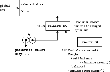
Now we can analyze what happens when
W1
is applied to an
argument:
(W1 50)
50
We begin by constructing a frame in which
amount
, the formal
parameter of
W1
, is bound to the argument 50. The crucial point
to observe is that this frame has as its enclosing environment not the
global environment, but rather the environment E1, because this is the
environment that is specified by the
W1
procedure object.
Within this new environment, we evaluate the body of the procedure:
(if (>= balance amount)
(begin (set! balance (- balance amount))
balance)
"Insufficient funds")
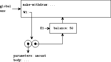
The resulting environment structure is shown in
figure
3.8
. The expression being evaluated references
both
amount
and
balance
.
Amount
will be found in
the first frame in the environment, while
balance
will be found
by following the enclosing-environment pointer to E1.
 |
When the
set!
is executed, the binding of
balance
in E1 is changed. At the completion of the call to
W1
,
balance
is 50, and the frame that contains
balance
is still pointed to by the procedure object
W1
. The frame
that binds
amount
(in which we executed the code that changed
balance
) is no longer
relevant, since the procedure call that constructed it has terminated,
and there are no pointers to that frame from other parts of the
environment. The next time
W1
is called, this will build a new
frame that binds
amount
and whose enclosing environment is E1.
We see that E1 serves as the “place” that holds the local state
variable for the procedure object
W1
. Figure
3.9
shows the situation after the call to
W1
.
 |
Observe what happens when we create a second “withdraw” object by
making another call to
make-withdraw
:
(define W2 (make-withdraw 100))
This produces the environment structure of figure
3.10
, which shows
that
W2
is a procedure object, that is, a pair with some code
and an environment. The environment E2 for
W2
was created by
the call to
make-withdraw
. It contains a frame with its own
local binding for
balance
. On the other hand,
W1
and
W2
have the same code: the code specified by the
lambda
expression in the body of
make-withdraw
.
15
We see here why
W1
and
W2
behave as independent objects. Calls to
W1
reference the state
variable
balance
stored in E1, whereas calls to
W2
reference the
balance
stored in E2. Thus, changes to the local
state of one object do not affect the other object.