Read Structure and Interpretation of Computer Programs Online
Authors: Harold Abelson and Gerald Jay Sussman with Julie Sussman
Structure and Interpretation of Computer Programs (50 page)

 |
Exercise 3.10.
In the
make-withdraw
procedure, the local variable
balance
is created as a parameter of
make-withdraw
. We could also
create the local state variable explicitly, using
let
, as
follows:
(define (make-withdraw initial-amount)
(let ((balance initial-amount))
(lambda (amount)
(if (>= balance amount)
(begin (set! balance (- balance amount))
balance)
"Insufficient funds"))))
Recall from section
1.3.2
that
let
is simply
syntactic sugar for a procedure call:
(let ((<
var
> <
exp
>)) <
body
>)
is interpreted as an alternate syntax for
((lambda (<
var
>) <
body
>) <
exp
>)
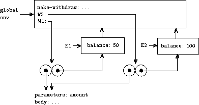
Use the environment model to analyze this alternate
version of
make-withdraw
, drawing figures like the ones above to
illustrate the interactions
(define W1 (make-withdraw 100))
(W1 50)
(define W2 (make-withdraw 100))
Show that the two versions of
make-withdraw
create objects with
the same behavior. How do the environment structures differ for the two
versions?
Section
1.1.8
introduced the idea that procedures can have internal
definitions, thus leading to a block structure as in the
following procedure to compute square roots:
(define (sqrt x)
(define (good-enough? guess)
(< (abs (- (square guess) x)) 0.001))
(define (improve guess)
(average guess (/ x guess)))
(define (sqrt-iter guess)
(if (good-enough? guess)
guess
(sqrt-iter (improve guess))))
(sqrt-iter 1.0))
Now we can use the environment model to see why these internal
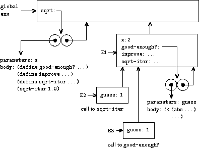
definitions behave as desired. Figure
3.11
shows the point in the
evaluation of the expression
(sqrt 2)
where the internal
procedure
good-enough?
has been called for the first time with
guess
equal to 1.
 |
Observe the structure of the environment.
Sqrt
is a symbol in
the global environment that is bound to a procedure object whose
associated environment is the global environment. When
sqrt
was
called, a new environment E1 was formed, subordinate to the global
environment, in which the parameter
x
is bound to 2. The body
of
sqrt
was then evaluated in E1. Since the first expression in
the body of
sqrt
is
(define (good-enough? guess)
(< (abs (- (square guess) x)) 0.001))
evaluating this expression defined the procedure
good-enough?
in the environment E1. To be more precise, the symbol
good-enough?
was added to the first frame of E1, bound to a
procedure object whose associated environment is E1. Similarly,
improve
and
sqrt-iter
were defined as procedures in E1. For
conciseness, figure
3.11
shows only the procedure
object for
good-enough?
.
After the local procedures were defined, the
expression
(sqrt-iter 1.0)
was evaluated,
still in environment E1. So the
procedure object bound to
sqrt-iter
in E1 was called with 1 as
an argument. This created an environment E2 in which
guess
,
the parameter of
sqrt-iter
, is bound to 1.
Sqrt-iter
in
turn called
good-enough?
with the value of
guess
(from
E2) as the argument for
good-enough?
. This set up another
environment, E3, in which
guess
(the parameter of
good-enough?
) is bound to 1. Although
sqrt-iter
and
good-enough?
both have a parameter named
guess
, these are two
distinct local variables located in different frames. Also, E2 and E3
both have E1 as their enclosing environment, because the
sqrt-iter
and
good-enough?
procedures both have E1 as their
environment part. One consequence of this is that the symbol
x
that appears in the body of
good-enough?
will reference the
binding of
x
that appears in E1, namely the value of
x
with which the original
sqrt
procedure was called.
The environment model thus explains the two key properties that make
local procedure definitions a useful technique for modularizing
programs:
- The names of the local procedures do not interfere with
names external to the enclosing procedure, because the local procedure
names will be bound in the frame that the procedure creates when it is
run, rather than being bound in the global environment. - The local procedures can access the arguments of the enclosing
procedure, simply by using parameter names as free variables.
This is because the body of the local procedure is evaluated in an
environment that is subordinate to the evaluation environment for the
enclosing procedure.
Exercise 3.11.
In section
3.2.3
we saw how the environment model described the
behavior of procedures with local state. Now we have seen how
internal definitions work. A typical message-passing procedure
contains both of these aspects. Consider the bank account procedure
of section
3.1.1
:
(define (make-account balance)
(define (withdraw amount)
(if (>= balance amount)
(begin (set! balance (- balance amount))
balance)
"Insufficient funds"))
(define (deposit amount)
(set! balance (+ balance amount))
balance)
(define (dispatch m)
(cond ((eq? m 'withdraw) withdraw)
((eq? m 'deposit) deposit)
(else (error "Unknown request -- MAKE-ACCOUNT"
m))))
dispatch)
Show the environment structure generated by the sequence of
interactions
(define acc (make-account 50))
((acc 'deposit) 40)
90
((acc 'withdraw) 60)
30
Where is the local state for
acc
kept? Suppose we define
another account
(define acc2 (make-account 100))
How are the local states for the two accounts kept distinct? Which
parts of the environment structure are shared between
acc
and
acc2
?
12
Assignment introduces a subtlety into step 1 of
the evaluation rule. As shown in
exercise
3.8
, the presence of assignment
allows us to write expressions that will produce different values
depending on the order in which the subexpressions in a combination
are evaluated. Thus, to be precise, we should specify an evaluation
order in step 1 (e.g., left to right or right to left). However, this
order should always be considered to be an implementation detail, and
one should never write programs that depend on some particular order.
For instance, a sophisticated compiler might optimize a program by
varying the order in which subexpressions are evaluated.
13
If there is already a binding for the
variable in the current frame, then the binding is changed. This is
convenient because it allows redefinition of symbols; however, it also
means that
define
can be used to change values, and this brings
up the issues of assignment without explicitly using
set!
.
Because of this, some people prefer redefinitions of existing symbols
to signal errors or warnings.
14
The
environment model will not clarify our claim in
section
1.2.1
that the interpreter can
execute a procedure such as
fact-iter
in a constant amount of
space using tail recursion. We will discuss tail recursion when we
deal with the control structure of the interpreter in
section
5.4
.
15
Whether
W1
and
W2
share the same physical code stored in the
computer, or whether they each keep a copy of the code, is a detail of
the implementation. For the interpreter we implement in chapter 4,
the code is in fact shared.
Chapter 2 dealt with compound data as a means for constructing
computational objects that have several parts, in order to model
real-world objects that have several aspects. In that chapter we
introduced the discipline of data abstraction, according to which data
structures are specified in terms of constructors, which create data
objects, and selectors, which access the parts of compound data
objects. But we now know that there is another aspect of data that
chapter 2 did not address. The desire to model systems composed of
objects that have changing state leads us to the need to modify
compound data objects, as well as to construct and select from them.
In order to model compound objects with changing state, we will design
data abstractions to include, in addition to selectors and
constructors, operations called
mutators
, which modify data
objects. For instance, modeling a banking system requires us to
change account balances. Thus, a data structure for representing bank
accounts might admit an operation
(set-balance! <
account
> <
new-value
>)
that changes the balance of the designated account to the designated
new value. Data objects for which mutators are defined are known as
mutable data objects
.
Chapter 2 introduced pairs as a general-purpose “glue” for
synthesizing compound data. We begin this section by defining basic
mutators for pairs, so that pairs can serve as building blocks for
constructing mutable data objects. These mutators greatly enhance the
representational power of pairs, enabling us to build data structures
other than the sequences and trees that we worked with in
section
2.2
. We also present some examples of
simulations in which complex systems are modeled as collections of
objects with local state.
The basic operations on pairs –
cons
,
car
, and
cdr
– can be used to construct list structure and to select parts
from list structure, but they are incapable of modifying list
structure. The same is true of the list operations we have used so
far, such as
append
and
list
, since these can be defined
in terms of
cons
,
car
, and
cdr
. To modify list
structures we need new operations.
 |
