Data Mining (112 page)
Authors: Mehmed Kantardzic

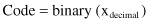
Figure 13.1.
Crossover operators. (a) One-point crossover; (b) two point crossover.
We can define an n-point crossover similarly, where the parts of strings between points 1 and 2, 3 and 4, and finally n-1 and n are swapped. The effect of crossover is similar to that of mating in the natural evolutionary process in which parents pass segments of their own chromosomes on to their children. Therefore, some children are able to outperform their parents if they get “good” genes or genetic traits from their parents.
13.2.5 Mutation
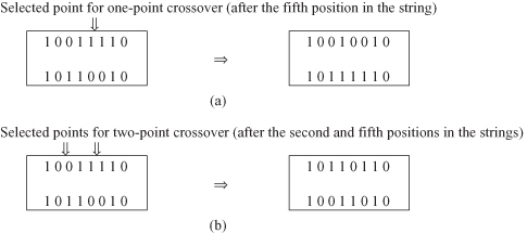
Crossover exploits existing gene potentials, but if the population does not contain all the encoded information needed to solve a particular problem, no amount of gene mixing can produce a satisfactory solution. For this reason, a mutation operator capable of spontaneously generating new chromosomes is included. The most common way of implementing mutation is to flip a bit with a probability equal to a very low given mutation rate (MR). A mutation operator can prevent any single bit from converging to a value through the entire population, and, more important, it can prevent the population from converging and stagnating at any local optima. The MR is usually kept low so good chromosomes obtained from crossover are not lost. If the MR is high (e.g., above 0.1), GA performance will approach that of a primitive random search. Figure
13.2
provides an example of mutation.
Figure 13.2.
Mutation operator.
In the natural evolutionary process, selection, crossover, and mutation all occur simultaneously to generate offspring. Here we split them into consecutive phases to facilitate implementation of and experimentation with GAs. Note that this section only gives a general description of the basics of GAs. Detailed implementations of GAs vary considerably, but the main phases and the iterative process remain.
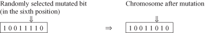
At the end of this section we can summarize that the major components of GA include encoding schemata, fitness evaluation, parent selection, and application of crossover operators and mutation operators. These phases are performed iteratively, as presented in Figure
13.3
.
Figure 13.3.
Major phases of a genetic algorithm.
It is relatively easy to keep track of the best individual chromosomes in the evolution process. It is customary in GA implementations to store “the best ever” individual at a separate location. In that way, the algorithm would report the best value found during the whole process, just in the final population.
Optimization under constraints is also the class of problems for which GAs are an appropriate solution. The constraint-handling techniques for genetic algorithms can be grouped into different categories. One typical way of dealing with GA candidates that violate the constraints is to generate potential solutions without considering the constraints, and then to penalize them by decreasing the “goodness” of the evaluation function. In other words, a constrained problem is transformed to an unconstrained one by associating a penalty with all constraint violations. These penalties are included in the function evaluation, and there are different kinds of implementations. Some penalty functions assign a constant as a penalty measure. Other penalty functions depend on the degree of violation: the larger the violation, the greater the penalty. The growth of the penalty function can be logarithmic, linear, quadratic, exponential, and so on, depending upon the size of the violation. Several implementations of GA optimization under constraints are given in the texts recommended for further study (Section 13.9).
13.3 A SIMPLE ILLUSTRATION OF A GA
To apply a GA for a particular problem, we have to define or to select the following five components:
1.
a genetic representation or encoding schema for potential solutions to the problem;
2.
a way to create an initial population of potential solutions;
3.
an evaluation function that plays the role of the environment, rating solutions in terms of their “fitness”;
4.
Genetic operators that alter the composition of the offspring; and
5.
values for the various parameters that the GA uses (population size, rate of applied operators, etc.).
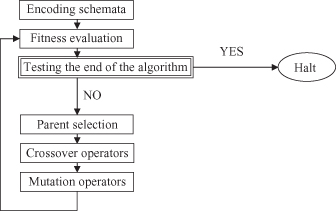
We discuss the main features of GAs by presenting a simple example. Suppose that the problem is the optimization of a simple function of one variable. The function is defined as

The task is to find x from the range [0,31], which maximizes the function f(x). We selected this problem because it is relatively easy to analyze optimization of the function f(x) analytically, to compare the results of the analytic optimization with a GA, and to find the approximate optimal solution.
13.3.1 Representation
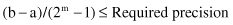
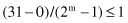
The first step in the GA is to represent the solution alternative (a value for the input feature) in a coded-string format. Typically, the string is a series of features with their values; each feature’s value can be coded with one from a set of discrete values called the allele set. The allele set is defined according to the needs of the problem, and finding the appropriate coding method is a part of the art of using GAs. The coding method must be minimal but completely expressive. We will use a binary vector as a chromosome to represent real values of the single variable x. The length of the vector depends on the required precision, which, in this example, is selected as 1. Therefore, we need a minimum five-bit code (string) to accommodate the range with required precision:


For this example, the mapping from a real number to a binary code is defined by the relation (because a = 0):