Data Mining (107 page)

Figure 12.34.
Joint probability distributions show different dependencies between variables
a
,
b
, and
c
.

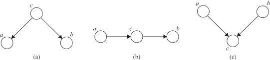
while for Figure
12.34
c the probability p(c| a, b) is under the assumption that variables
a
and
b
are independent
p
(
a, b
) =
p
(
a
) p(
b
).

In general, graphical models may capture the
causal
processes by which the observed data were generated. For this reason, such models are often called
generative
models. We could make previous models in Figure
12.33
generative by introducing a suitable prior distribution p(x) for all input variables (these are variables—nodes without input links). For the case in Figure
12.33
a this is a variable
a
, and for the case in Figure
12.33
b these are variables: x
₁
, x
₂
, and x
₃
. In practice, producing synthetic observations from a generative model can prove informative in understanding the form of the probability distribution represented by that model.

This preliminary analysis about joint probability distributions brings us to the concept of Bayesian networks (BN).
BN
are also called belief networks or probabilistic networks in the literature. The nodes in a BN represent variables of interest (e.g., the temperature of a device, the gender of a patient, the price of a product, the occurrence of an event), and the links represent dependencies among the variables. Each node has
states
, or a set of probable values for each variable. For example, the weather could be cloudy or sunny, an enemy battalion could be near or far, symptoms of a disease are present or not present, and the garbage disposal is working or not working. Nodes are connected with an arrow to show causality and also indicate the direction of influence. These arrows are called
edges
. The dependencies are quantified by conditional probabilities for each node given its parents in the network. Figure
12.35
presents some BN architectures, initially without probabilities distributions. In general, we can formally describe a BN as a graph in which the following holds:

Figure 12.35.
Two examples of Bayesian network architectures.

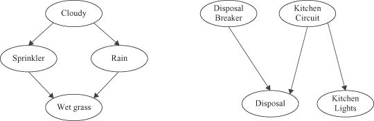
Each node in the BN corresponds to a random variable X, and has a probability distribution of the variable P(X). If there is a directed arc from node X to node Y, this indicates that X has a direct influence on Y. The influence is specified by the conditional probability P(Y|X). Nodes and arcs define a
structure
of the BN. Probabilities are
parameters
of the structure.

We turn now to the problem of inference in graphical models, in which some of the nodes in a graph are clamped to observed values, and we wish to compute the posterior distributions of one or more subsets of other nodes. The network supports the computation of the probabilities of any subset of variables given evidence about any other subset. We can exploit the graphical structure both to find efficient algorithms for inference and to make the structure of those algorithms transparent. Specifically, many inference-based algorithms can be expressed in terms of the propagation of local
probabilities
around the graph. A BN can be considered as a probabilistic graph in which the probabilistic knowledge is represented by the topology of the network and the conditional probabilities at each node. The main purpose of building knowledge on probabilities is to use it for inference, that is, for computing the answer for particular cases about the domain.

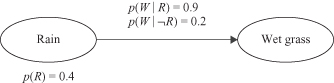
For example, we may assume that rain causes the grass to get wet. Causal graph in Figure
12.36
explains the cause–effect relation between these variables, including corresponding probabilities. If P(Rain) = P(R) = 0.4 is given, that also means P(
R) = 0.6. Also, note that the sum of presented conditional probabilities is not equal to 1. If you analyze the relations between probabilities, P(W|R) + P(
W|R) = 1, and also P(W|
R) + P(
W|
R) = 1, not the sum of given probabilities. In these expressions R means “Rain,” and W means “Wet grass.” Based on the given BN, we may check the probability of “Wet grass”:

Figure 12.36.
Simple causal graph.

Bayes’ rule allows us to invert the dependencies, and obtain probabilities of parents in the graph based on probabilities of children. That could be useful in many applications, such as determining probability of a diagnosis based on symptoms. For example, based on the BN in Figure
12.36
, we may determine conditional probability P(Rain|Wet grass) = P(R|W). We know that