Data Mining (105 page)

So, instead of sending an m-dimensional vector to the other site, the algorithm sends only a (k + 1)-dimensional vector where k
m (k is a user-defined parameter). The inner product of vectors can still be estimated accurately with lower communication load.

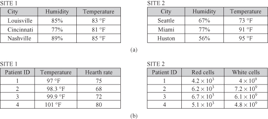
In the DDM literature, one of two assumptions is commonly adopted as to how data are distributed across sites: (1) homogeneously or horizontally partitioned, or (2) heterogeneously or vertically partitioned. Both viewpoints assume that the data tables at each distributed site are partitions of a single global table. It is important to stress that the global table viewpoint is strictly conceptual. It is not necessarily assumed that such a table was physically realized and partitioned to form the tables at each site. In the homogeneous case, the global table is horizontally partitioned. The tables at each site are subsets of the global table; they have exactly the same attributes. Figure
12.30
a illustrates the homogeneously distributed case using an example from weather data where both tables use the same three attributes. In the heterogeneous case, the table is vertically partitioned where each site contains a subset of columns. That means sites do not have the same attributes. However, samples at each site are assumed to contain a unique identifier to facilitate matching, and Figure
12.30
b illustrates this case. The tables at distributed sites have different attributes, and samples are linked through a unique identifier, Patient ID.

Figure 12.30.
Horizontally versus vertically partitioned data. (a) Horizontally partitioned data; (b) vertically partitioned data.

DDM technology supports different data-mining tasks including classification, prediction, clustering, market-basket analysis, and outliers’ detection. A solution for each of these tasks may be implemented with a variety of DDM algorithms. For example, distributed Apriori has several versions for frequent itemset generation in distributed transactional database. They usually require multiple synchronizations and communication steps. Most of these implementations assume that platforms are homogeneous and therefore the data sets are partitioned evenly among the sites. However, in practice, both the data sets and the processing platforms are more likely to be heterogeneous, running multiple and different systems and tools. This leads to unbalanced data-set distributions and workloads causing additional problems in implementation.

One recent trend is online-mining technology used for monitoring in distributed sensor networks. This is because deployments of large-scale distributed sensor networks are now possible owing to hardware advances and increasing software support. Online data mining, also called
data-stream mining
, is concerned with extracting patterns, detecting outliers, or developing dynamic models of a system’s behavior from continuous data streams such as those generated by sensor networks. Because of the massive amount of data and the speed of which the data are generated, many data-mining applications in sensor networks require in-network processing such as aggregation to reduce sample size and communication overhead. Online data mining in sensor networks offers many additional challenges, including:

• limited communication bandwidth,
  
• constraints on local computing resources,
  
• limited power supply,
  
• need for fault tolerance, and
  
• asynchronous nature of the network.
  

Obviously, data-mining systems have evolved in a short period of time from stand-alone programs characterized by single algorithms with little support for the entire knowledge-discovery process to integrated systems incorporating several mining algorithms, multiple users, communications, and various and heterogeneous data formats and distributed data sources. Although many DDM algorithms are developed and deployed in a variety of applications, the trend will be illustrated in this book with only one example of a distributed clustering algorithm.

12.4.1 Distributed DBSCAN Clustering

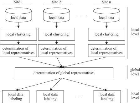
Distributed clustering assumes that samples to be clustered reside on different sites. Instead of transmitting all samples to a central site where we can apply one of the standard clustering algorithms to analyze the data locally, the data are clustered independently on the distributed local sites. Then, in a subsequent step, the central site tries to establish a global clustering model based on the downloaded local models, that is, summarized representatives of local data. Distributed clustering is carried out on two different levels, that is, the local level and the global level (Fig.
12.31
). On the local level, all sites carry out clustering independently from each other. Communication with the central site and determining a global model should reflect an optimum trade-off between complexity and accuracy of the algorithm.

Figure 12.31.
System architecture for distributed clustering.

Local models consist of a set of representatives for each locally found cluster. A representative is a good approximation for samples residing on the corresponding local site. The local model is transferred to a central site, where the local models are merged in order to form a global model. The representation of local models should be simple enough so there will be no overload in communications. At the same time, local models should be informative enough to support a high quality of approximate global clustering. The global model is created by analyzing and integrating local representatives. The resulting global clustering is sent back, at the end of the process, to all local sites.

This global-distributed framework may be more precisely specified when we implement a specific clustering algorithm. The density-based clustering algorithm DBSCAN is a good candidate, because it is robust to outliers, easy to implement, supports clusters of different shapes, and allows incremental, online implementation. The main steps of the algorithm are explained in Chapter 9, and the same process is applied locally. To find local clusters, DBSCAN starts with an arbitrary core object
p
, which is not yet clustered and retrieves all objects density reachable from
p
. The retrieval of density-reachable objects is performed in iterations until all local samples are analyzed. After having clustered the data locally, we need a small number of representatives that will describe the local clustering result accurately. For determining suitable representatives of the clusters, the concept of
specific core points
is introduced.

Let C be a local cluster with respect to the given DBSCAN parameters ε and
MinPts
. Furthermore, let
Cor
_C
⊆
C
be the set of core points belonging to this cluster. Then
Scor
_C
⊆
C
is called a
complete set of specific core points of C
iff the following conditions are true:

• Scor
  _C
  ⊆
  Cor
  _C
  
• ∀
  s
  _i
  ,s
  _j
  ⊆
  Scor
  _C
  : s
  _i
  ∉
  Neighborhood
  _ε
  (
  s
  _j
  )
  
• ∀
  c
  ∈
  Cor
  _C
  ,
  ∃
  s
  ∈
  Scor
  _C
  : c
  ∈
  Neighborhood
  _ε
  (
  s)
  

The
Scor
_C
set of points consists of a very small number of
specific core points
that describe the cluster
C
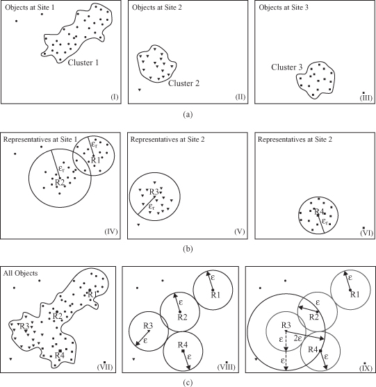
. For example, in Figure
12.32
a, sites 2 and 3 have only one
specific core point
, while site 1, because of the cluster shape, has two
specific core points.
To further simplify the representation of local clusters, the number of specific core points, |
Scor
_C
| = K, is used as an input parameter for a further local “clustering step” with an adapted version of
K-means
. For each cluster
C
found by
DBSCAN
, k-means use
Scor
_C
points as starting points. The result is K = |
Scor
_C
| subclusters and centroids within
C
.

Figure 12.32.
Distributed DBSCAN clustering

(Januzaj et al., 2003).

(a) Local clusters; (b) local representatives; (c) global model with ε
_global
=
2
ε
_local
.

Each local model
LocalModel
_k
consists of a set of
m
_k
pairs: a representative
r
(complete specific core point), and an ε radius value. The number
m
of pairs transmitted from each site
k
is determined by the number
n
of clusters
C
_i
found on site
k.
Each of these pairs (
r
, ε
_r
) represents a subset of samples that are all located in a corresponding local cluster. Obviously, we have to check whether it is possible to merge two or more of these clusters, found on different sites, together. That is the main task of a global modeling part. To find such a global model, the algorithm continues with the density-based clustering algorithm DBSCAN again but only for collected representatives from local models. Because of characteristics of these representative points, the parameter
MinPts
_global
is set to 2, and radius ε
_global
value should be set generally close to
2
ε
_local
.

In Figure
12.32
, an example of distributed DBSCAN for ε
_global
=
2
ε
_local
is depicted. In Figure
12.32
a the independently detected clusters on site 1, 2, and 3 are represented. The cluster on site 1 is represented using K-means by two representatives,
R
₁
and
R
₂
, whereas the clusters on site 2 and site 3 are only represented by one representative as shown in Figure
12.32
b. Figure
12.32
c illustrates that all four local clusters from the different sites are merged together in one large cluster. This integration is obtained by using an ε
_global
parameter equal to
2
ε
_local
. Figure
12.32
c also makes clear that an ε
_global
= ε
_local
is insufficient to detect this global cluster. When the final global model is obtained, the model is distributed to local sites. This model makes corrections comparing previously found local models. For example, in the local clustering some points may be left as outliers, but with the global model they may be integrated into modified clusters.