Authors: Mehmed Kantardzic
Data Mining (101 page)

and normalized similarity measure is

In order to deal with noise, scaling, approximate values, and translation problems, a simple improvement consists of determining the pairs of sequence portions that agree in both sequences after some linear transformations are applied. It consists of determining if there is a linear function
f
, such that one sequence can be approximately mapped into the other. In most applications involving determination of similarity between pairs of sequences, the sequences would be of different lengths. In such cases, it is not possible to blindly accumulate distances between corresponding elements of the sequences. This brings us to the second aspect of sequence matching, namely, sequence alignment. Essentially, we need to properly insert “gaps” in the two sequences or decide which should be corresponding elements in the two sequences. There are many situations in which such symbolic sequence matching problems find applications. For example, many biological sequences such as genes and proteins can be regarded as sequences over a finite alphabet. When two such sequences are similar, it is expected that the corresponding biological entities have similar functions because of related biochemical mechanisms. The approach includes a similarity measure for sequences based on the concept of the edit distance for strings of discrete symbols. This distance reflects the amount of work needed to transform a sequence to another, and is able to deal with different sequences length and gaps existence. Typical edit operations are insert, delete, and replace, and they may be included in the measure with the same or with different weights (costs) in the transformation process. The distance between two strings is defined as the least sum of edit operation costs that needs to be performed to transform one string into another. For example, if two sequences are given: X = {a, b, c, b, d, a, b, c} and Y = { b, b, b, d, b}, the following operations are applied to transform X into Y: delete (a), replace (c,b), delete (a), delete (c). The total number of operations in this case is four, and it represents non-normalized distance measure between two sequences.
12.2.3 Temporal Data Modeling
A
model
is a global, high-level, and often abstract representation of data. Typically, models are specified by a collection of model parameters that can be estimated from a given data set. It is possible to classify models as predictive or descriptive depending on the task they are performing. In contrast to the (global) model structure, a
temporal pattern
is a local model that makes a specific statement about a few data samples in time. Spikes, for example, are patterns in a real-valued time series that may be of interest. Similarly, in symbolic sequences, regular expressions represent well-defined patterns. In bioinformatics, genes are known to appear as local patterns interspersed between chunks of noncoding DNA. Matching and discovery of such patterns are very useful in many applications, not only in bioinformatics. Due to their readily interpretable structure, patterns play a particularly dominant role in data mining. There have been many techniques used to model global or local temporal events. We will introduce only some of the most popular modeling techniques.
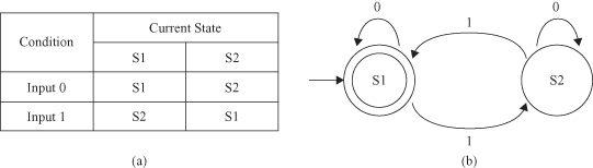
Finite State Machine (FSM)
has a set of states and a set of transitions. A state may have transitions to other states that are caused by fulfilling some conditions within the state. An FSM must have an initial state, usually drawn with an arrow, and it is a state that provides a starting point of the model. Inputs to the states, in our case representing symbols in a sequence, act as triggers for the transition from one state to another state. An accept state, which is also known as final state, is usually represented by a double circle in a graph representation. The machine reaches the final state when it has performed the procedure successfully, or in our case recognized a sequence pattern. An FSM can be represented using a state-transition table or state-transition diagram. Figures
12.20
a,b shows both of these representations for a modeling recognition of a binary number with an even number of ones. FSM does not work very well when the transitions are not precise and does not scale well when the set of symbols for sequence representation is large.
Figure 12.20.
Finite-state machine. (a) State-transition table; (b) state-transition diagram.
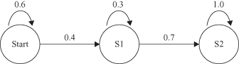
Markov Model (MM)
extends the basic idea behind FSM. Both FSM and MM are directed graphs. As with FSM, MM always has a current state. Start and end nodes are drawn for illustrative purposes and need not be present. Unlike in FSM, transitions are not associated with specific input values. Arcs carry a probability value for transition from one state to another. For example, the probability that transition from state “Start” to “S1” is 0.4 and the probability of staying in the “Start” state is 0.6. The sum of the probability values coming out of each node should be 1. MM shows only transitions with probability greater than 0. If a transition is not shown, it is assumed to have a probability of 0. The probabilities are combined to determine the final probability of the pattern produced by the MM. For example, with the MM shown in Figure
12.21
, the probability that the MM takes the horizontal path from starting node to S2 is 0.4 × 0.7 = 0.28.
Figure 12.21.
A simple Markov Model.
MM is derived based on the memoryless assumption. It states that given the current state of the system, the future evolution of the system is independent of its history. MMs have been used widely in speech recognition and natural language processing.
Hidden Markov Model (HMM)
is an extension to MM. Similar to MM, HMM consists of a set of states and transition probabilities. In a regular MM, the states are visible to the observer, and the state-transition probabilities are the only parameters. In HMM, each state is associated with a state-probability distribution. For example, assume that we were given a sequence of events in a coin toss: O = (HTTHTHH), where H = Head and T = Tail. But additional information is necessary. What is not given is the sequence generated with one or two coins. According to the above definitions, Figure
12.22
shows two possible models. Figure
12.22
a assumes that only one coin was tossed. We can model this system as an MM with a two-state model, where Head and Tail are the two states with the same initial probabilities. The probability of the sequence O is P(O) = 0.5 × 0.7 × 0.3 × 0.7 × 0.3 × 0.7 × 0.7 = 0.0108.
Figure 12.22.
Markov Model versus hidden Markov Model. (a) One-coin model; (b) two-coin model.
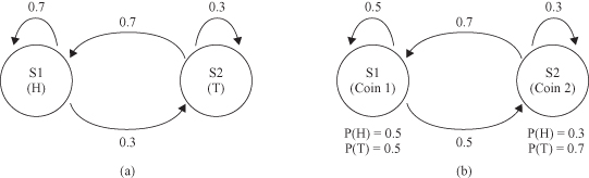
Another possibility for explaining the observed sequence is shown in Figure
12.22
b. There are again two states in this model, and each state corresponds to a separate biased coin being tossed. Each state has its own probability distribution of Heads and Tails, and therefore the model is represented as an HMM. Obviously, in this model we have several “paths” to determine the probability of the sequence. In other words, we can start with tossing one or another coin, and continue with this selection. In all these cases, composite probability will be different. In this situation, we may search for the maximum probability of the sequence O in the HMM. HMM may be formalized as a directed graph with
V
vertices and
A
arcs. Set V = {v
1
, v
2
, … , v
n
} represents states, and matrix A = {a
ij
} represents transition-probability distribution, where a
ij
is the transitional probability from state i to state j. Given a set of possible observations O = {o
1
, o
2
, … , o
m
} for each state v
i
, the probability of seeing each observation in the sequence is given by Bi = {o
i1
, o
i2
, … , o
im
}. The initial-state distribution is represented as σ, which determines the starting state at time
t
= 0.
12.2.4 Mining Sequences
Temporal data-mining tasks include prediction, classification, clustering, search and retrieval, and pattern discovery. The first four have been investigated extensively in traditional time-series analysis, pattern recognition, and information retrieval. We will concentrate in this text on illustrative examples of algorithms for pattern discovery in large databases, which are of more recent origin and showing wide applicability. The problem of pattern discovery is to find and evaluate all “interesting” patterns in the data. There are many ways of defining what constitutes a pattern in the data and we shall discuss some generic approaches. There is no universal notion for interestingness of a pattern either. However, one concept that is found very useful in data mining is that of frequent patterns. A frequent pattern is one that occurs many times in the data. Much of the data-mining literature is concerned with formulating useful pattern structures and developing efficient algorithms for discovering all patterns that occur frequently in the data.
A pattern is a local structure in the database. In the sequential-pattern framework, we are given a collection of sequences, and the task is to discover sequences of items called sequential patterns that occur in sufficiently many of those sequences. In the frequent episodes analysis, the data set may be given in a single long sequence or in a large set of shorter sequences. An
event sequence
is denoted by {(
E
1
,
t
1
), (
E
2
,
t
2
),
…
, (
E
n
,
,
t
n
)}, where
E
i
takes values from a finite set of event types
E
, and
t
i
is an integer denoting the time stamp of the
i
th
event. The sequence is ordered with respect to the time stamps so that
t
i
≤
t
i
+
1
for all
i
= 1, 2, … ,
n.
The following is an example event sequence S with 10 events in it: