Authors: Mehmed Kantardzic
Data Mining (103 page)

Ubiquitous Data Mining (UDM) is an additional new field that defines a process of performing analysis of data on mobile, embedded, and ubiquitous devices. It represents the next generation of data-mining systems that will support the intelligent and time-critical information needs of mobile users and will facilitate “anytime, anywhere” data mining. It is the next natural step in the world of ubiquitous computing. The underlying focus of UDM systems is to perform computationally intensive mining techniques in mobile environments that are constrained by limited computational resources and varying network characteristics. Additional technical challenges are as follows: How to minimize energy consumption of the mobile device during the data mining process; how to present results on relatively small screens; and how to transfer data mining results over a wireless network with a limited bandwidth?
12.3 SPATIAL DATA MINING (SDM)
SDM is the process of discovering interesting and previously unknown but potentially useful information from large spatial data sets. Spatial data carries topological and/or distance information, and it is often organized in databases by spatial indexing structures and accessed by spatial access methods. The applications covered by SDM include geomarketing, environmental studies, risk analysis, remote sensing, geographical information systems (GIS), computer cartography, environmental planning, and so on. For example, in geomarketing, a store can establish its trade area, that is, the spatial extent of its customers, and then analyze the profile of those customers on the basis of both their properties and the area where they live. Simple illustrations of SDM results are given in Figure
12.25
, where (a) shows that a fire is often located close to a dry tree and a bird is often seen in the neighborhood of a house, while (b) emphasizes a significant trend that can be observed for the city of Munich, where the average rent decreases quite regularly when moving away from the city. One of the main reasons for developing a large number of spatial data-mining applications is the enormous amount of special data that are collected recently at a relatively low price. High spatial and spectral resolution remote-sensing systems and other environmental monitoring devices gather vast amounts of geo-referenced digital imagery, video, and sound. The complexity of spatial data and intrinsic spatial relationships limits the usefulness of conventional data-mining techniques for extracting spatial patterns.
Figure 12.25.
Illustrative examples of spatial data-mining results. (a) Example of collocation spatial data mining
(Shekhar and Chawla, 2003);
(b) average rent for the communities of Bavaria
(Ester et al., 1997).
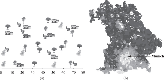
Figure 12.26.
Main differences between traditional data mining and spatial data mining.
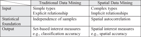
One of the fundamental assumptions of data-mining analysis is that the data samples are independently generated. However, in the analysis of spatial data, the assumption about the independence of samples is generally false. In fact, spatial data tends to be highly self-correlated. Extracting interesting and useful patterns from spatial data sets is more difficult than extracting corresponding patterns from traditional numeric and categorical data due to the complexity of spatial data types, spatial relationships, and spatial autocorrelation. The spatial attributes of a spatial object most often include information related to spatial locations, for example, longitude, latitude and elevation, as well as shape. Relationships among nonspatial objects are explicit in data inputs, for example, arithmetic relation, ordering, is an instance of, subclass of, and membership of. In contrast, relationships among spatial objects are often implicit, such as overlap, intersect, close, and behind. Proximity can be defined in highly general terms, including distance, direction and/or topology. Also, spatial heterogeneity or the nonstationarity of the observed variables with respect to location is often evident since many space processes are local. Omitting the fact that nearby items tend to be more similar than items situated apart causes inconsistent results in the spatial data analysis. In summary, specific features of spatial data that preclude the use of general-purpose data-mining algorithms are: (1) rich data types (e.g., extended spatial objects), (2) implicit spatial relationships among the variables, (3) observations that are not independent, and (4) spatial autocorrelation among the features (Fig.
12.26
).
One possible way to deal with implicit spatial relationships is to materialize the relationships into traditional data input columns and then apply classical data-mining techniques. However, this approach can result in loss of information. Another way to capture implicit spatial relationships is to develop models or techniques to incorporate spatial information into the spatial data-mining process. A concept within statistics devoted to the analysis of spatial relations is called spatial autocorrelation. Knowledge-discovery techniques, which ignore spatial autocorrelation, typically perform poorly in the presence of spatial data.
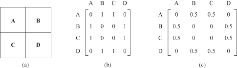
The spatial relationship among locations in a spatial framework is often modeled via a contiguity matrix. A simple contiguity matrix may represent a neighborhood relationship defined using adjacency. Figure
12.27
a shows a gridded spatial framework with four locations, A, B, C, and D. A binary matrix representation of a four-neighborhood relationship is shown in Figure
12.27
b. The row-normalized representation of this matrix is called a contiguity matrix, as shown in Figure
12.27
c. The essential idea is to specify the pairs of locations that influence each other along with the relative intensity of interaction.
Figure 12.27.
Spatial framework and its four-neighborhood contiguity matrix.
SDM consists of extracting knowledge, spatial relationships, and any other properties that are not explicitly stored in the database. SDM is used to find implicit regularities, and relations between spatial data and/or nonspatial data. In effect, a spatial database constitutes a spatial continuum in which properties concerning a particular place are generally linked and explained in terms of the properties of its neighborhood. In this section, we introduce as illustrations of SDM two important characteristics and often used techniques: (1) spatial autoregressive (SAR) modeling, and (2) spatial outliers’ detection using variogram-cloud technique.
1.
The SAR model
is a classification technique that decomposes a classifier into two parts, spatial autoregression and logistic transformation. Spatial dependencies are modeled using the framework of logistic regression analysis. If the spatially dependent values y
i
are related to each other, then the traditional regression equation can be modified as
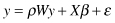
where
W
is the neighborhood relationship contiguity matrix and
ρ
is a parameter that reflects the strength of the spatial dependencies between the elements of the dependent variable. After the correction term
ρWy
is introduced, the components of the residual error vector ε are then assumed to be generated from independent and identical standard normal distributions. As in the case of classical regression, the proposed equation has to be transformed via the logistic function for binary dependent variables, and we refer to this equation as the SAR model. Notice that when
ρ
= 0, this equation collapses to the classical regression model. If the spatial autocorrelation coefficient is statistically significant, then SAR will quantify the presence of spatial autocorrelation in the classification model. It will indicate the extent to which variations in the dependent variable (
y
) are influenced by the average of neighboring observation values.
2.
A spatial outlier
is a spatially referenced object whose nonspatial attribute values differ significantly from those of other spatially referenced objects in its spatial neighborhood. This kind of outlier shows a local instability in values of nonspatial attributes. It represents spatially referenced objects whose nonspatial attributes are extreme relative to its neighbors, even though the attributes may not be significantly different from the entire population. For example, a new house in an old neighborhood of a growing metropolitan area is a spatial outlier based on the nonspatial attribute house age.
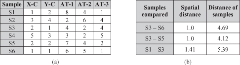
A variogram-cloud technique displays data points related by neighborhood relationships. For each pair of samples, the square-root of the absolute difference between attribute values at the locations versus the Euclidean distance between the locations is plotted. In data sets exhibiting strong spatial dependence, the variance in the attribute differences will increase with increasing distance between locations. Locations that are near to one another, but with large attribute differences, might indicate a spatial outlier, even though the values at both locations may appear to be reasonable when examining the dataset nonspatially. For example, the spatial data set is represented with six five-dimensional samples given in Figure
12.28
a. Traditional nonspatial analysis will not discover any outliers especially because the number of samples is relatively small. However, after applying a variogram-cloud technique, assuming that the first two attributes are X-Y spatial coordinates, and the other three are characteristics of samples, the conclusion could be significantly changed. Figure
12.29
shows the variogram-cloud for this data set. This plot has some pairs of points that are out of main dense region of common distances.
Figure 12.28.
An example of a variogram-cloud graph. (a) Spatial data set; (b) a critical sample’s relations in a variogram-cloud.