Data Mining (50 page)
Authors: Mehmed Kantardzic

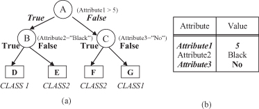
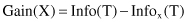
Figure 6.3.
Classification of a new sample based on the decision-tree model. (a) Decision tree; (b) An example for classification.
The skeleton of the C4.5 algorithm is based on Hunt’s Concept Learning System (CLS) method for constructing a decision tree from a set T of training samples. Let the classes be denoted as {C
1
, C
2
, … , C
k
}. There are three possibilities for the content of the set T:
1.
T contains one or more samples, all belonging to a single class C
j
. The decision tree for T is a leaf-identifying class C
j
.
2.
T contains no samples. The decision tree is again a leaf but the class to be associated with the leaf must be determined from information other than T, such as the overall majority class in T. The C4.5 algorithm uses as a criterion the most frequent class at the parent of the given node.
3.
T contains samples that belong to a mixture of classes. In this situation, the idea is to refine T into subsets of samples that are heading toward a single-class collection of samples. Based on single attribute, an appropriate test that has one or more mutually exclusive outcomes {O
1
, O
2
, … , O
n
} is chosen. T is partitioned into subsets T
1
, T
2
, … , T
n
, where T
i
contains all the samples in T that have outcome O
i
of the chosen test. The decision tree for T consists of a decision node identifying the test and one branch for each possible outcome (examples of this type of nodes are nodes A, B, and C in the decision tree in Fig.
6.3
a).
The same tree-building procedure is applied recursively to each subset of training samples, so that the
i
th branch leads to the decision tree constructed from the subset T
i
of the training samples. The successive division of the set of training samples proceeds until all the subsets consist of samples belonging to a single class.
The tree-building process is not uniquely defined. For different tests, even for a different order of their application, different trees will be generated. Ideally, we would like to choose a test at each stage of sample-set splitting so that the final tree is small. Since we are looking for a compact decision tree that is consistent with the training set, why not explore all possible trees and select the simplest? Unfortunately, the problem of finding the smallest decision tree consistent with a training data set is NP-complete. Enumeration and analysis of all possible trees will cause a combinatorial explosion for any real-world problem. For example, for a small database with five attributes and only 20 training examples, the possible number of decision trees is greater than 10
6
, depending on the number of different values for every attribute. Therefore, most decision tree-construction methods are non-backtracking, greedy algorithms. Once a test has been selected using some heuristics to maximize the measure of progress and the current set of training cases has been partitioned, the consequences of alternative choices are not explored. The measure of progress is a local measure, and the gain criterion for a test selection is based on the information available for a given step of data splitting.
Suppose we have the task of selecting a possible test with n outcomes (n values for a given feature) that partitions the set T of training samples into subsets T
1
, T
2
, … , T
n
. The only information available for guidance is the distribution of classes in T and its subsets T
i
. If S is any set of samples, let
freq
(C
i
, S) stand for the number of samples in S that belong to class C
i
(out of k possible classes), and let |S| denote the number of samples in the set S.
The original ID3 algorithm used a criterion called
gain
to select the attribute to be tested that is based on the information theory concept:
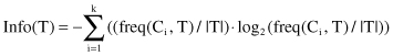
entropy
. The following relation gives the computation of the entropy of the set T (bits are units):
Now consider a similar measurement after T has been partitioned in accordance with n outcomes of one attribute test X. The expected information requirement can be found as the weighted sum of entropies over the subsets:
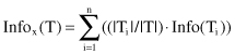
The quantity
measures the information that is gained by partitioning T in accordance with the test X. The gain criterion selects a test X to maximize Gain(X), that is, this criterion will select an attribute with the highest information gain.
Let us analyze the application of these measures and the creation of a decision tree for one simple example. Suppose that the database T is given in a flat form in which each of 14 examples (cases) is described by three input attributes and belongs to one of two given classes: CLASS1 or CLASS2. The database is given in tabular form in Table
6.1
.
TABLE 6.1.
A Simple Flat Database of Examples for Training
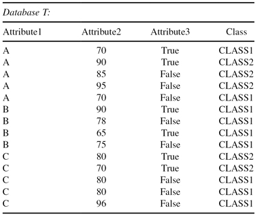
Nine samples belong to CLASS1 and five samples to CLASS2, so the entropy before splitting is

After using Attribute1 to divide the initial set of samples T into three subsets (test x
1
represents the selection one of three values A, B, or C), the resulting information is given by:
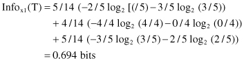
The information gained by this test x
1
is

If the test and splitting is based on Attribute3 (test x
2
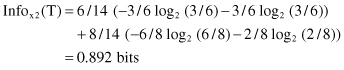
represents the selection one of two values True or False), a similar computation will give new results: