Data Mining (53 page)
Authors: Mehmed Kantardzic

Additionally, the concept of partitioning must be generalized. With every sample a new parameter, probability, is associated. When a case with known value is assigned from T to subset T
i
, the probability of it belonging to T
i
is 1, and in all other subsets is 0. When a value is not known, only a weaker probabilistic statement can be made. C4.5 therefore associates with each sample (having a missing value) in each subset T
i
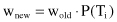
a weight w, representing the probability that the case belongs to each subset. To make the solution more general, it is necessary to take into account that the probabilities of samples before splitting are not always equal to one (in subsequent iterations of the decision-tree construction). Therefore, new parameter w
new
for missing values after splitting is equal to the old parameter w
old
before splitting multiplied by the probability that the sample belongs to each subset P(T
i
), or more formally:
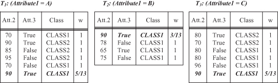
For example, the record with the missing value, given in the database in Figure
6.7
, will be represented in all three subsets after the splitting set T into subsets T
i
using test x
1
on Attribute1. New weights w
i
will be equal to probabilities 5/13, 3/13, and 5/13, because the initial (old) value for w is equal to one. The new subsets are given in Figure
6.7
. |T
i
| can now be reinterpreted in C4.5 not as a number of elements in a set T
i
, but as a sum of all weights w for the given set T
i
. From Figure
6.7
, the new values are computed as: |T
1
| = 5 + 5/13, |T
2
| = 3 + 3/13, and |T
3
| = 5 + 5/13.
Figure 6.7.
Results of test x
1
are subsets T
i
(initial set T is with missing value).
If these subsets are partitioned further by the tests on Attribute2 and Attribute3, the final decision tree for a data set with missing values has the form shown in Figure
6.8
Figure 6.8.
Decision tree for the database T with missing values.
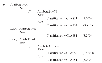
The decision tree in Figure
6.8
has much the same structure as before (Fig.
6.6
), but because of the ambiguity in final classification, every decision is attached with two parameters in a form (|T
i
|/E). |T
i
| is the sum of the fractional samples that reach the leaf and E is the number of samples that belong to classes other than the nominated class.
For example, (3.4/0.4) means that 3.4 (or 3 + 5/13) fractional training samples reached the leaf, of which 0.4 (or 5/13) did not belong to the class assigned to the leaf. It is possible to express the |T
i
| and E parameters in percentages:


A similar approach is taken in C4.5 when the decision tree is used to classify a sample previously not present in a database, that is, the
testing phase
. If all attribute values are known then the process is straightforward. Starting with a root node in a decision tree, tests on attribute values will determine traversal through the tree, and at the end, the algorithm will finish in one of the leaf nodes that uniquely define the class of a testing example (or with probabilities, if the training set had missing values). If the value for a relevant testing attribute is unknown, the outcome of the test cannot be determined. Then the system explores all possible outcomes from the test and combines the resulting classification arithmetically. Since there can be multiple paths from the root of a tree or subtree to the leaves, a classification is a class distribution rather than a single class. When the total class distribution for the tested case has been established, the class with the highest probability is assigned as the predicted class.
6.4 PRUNING DECISION TREES
Discarding one or more subtrees and replacing them with leaves simplify a decision tree, and that is the main task in decision-tree pruning. In replacing the subtree with a leaf, the algorithm expects to lower the
predicted error rate and
increase the quality of a classification model. But computation of error rate is not simple. An error rate based only on a training data set does not provide a suitable estimate. One possibility to estimate the predicted error rate is to use a new, additional set of test samples if they are available, or to use the cross-validation techniques explained in Chapter 4. This technique divides initially available samples into equal-sized blocks and, for each block, the tree is constructed from all samples except this block and tested with a given block of samples. With the available training and testing samples, the basic idea of decision tree pruning is to remove parts of the tree (subtrees) that do not contribute to the classification accuracy of unseen testing samples, producing a less complex and thus more comprehensible tree. There are two ways in which the recursive-partitioning method can be modified:
1.
Deciding Not to Divide a Set of Samples Any Further under Some Conditions.
The stopping criterion is usually based on some statistical tests, such as the χ
2
test: If there are no significant differences in classification accuracy before and after division, then represent a current node as a leaf. The decision is made in advance, before splitting, and therefore this approach is called
prepruning
.
2.
Removing Retrospectively Some of the Tree Structure Using Selected Accuracy Criteria.
The decision in this process of
postpruning
is made after the tree has been built.
C4.5 follows the
postpruning
approach, but it uses a specific technique to estimate the predicted error rate. This method is called
pessimistic pruning
. For every node in a tree, the estimation of the upper confidence limit U
cf
is computed using the statistical tables for binomial distribution (given in most textbooks on statistics). Parameter U
cf
is a function of |T
i
| and E for a given node. C4.5 uses the default confidence level of 25%, and compares U
25%
(|T
i
|/E) for a given node T
i
with a weighted confidence of its leaves. Weights are the total number of cases for every leaf. If the predicted error for a root node in a subtree is less than weighted sum of U
25%
for the leaves (predicted error for the subtree), then a subtree will be replaced with its root node, which becomes a new leaf in a pruned tree.
Let us illustrate this procedure with one simple example. A subtree of a decision tree is given in Figure
6.9
, where the root node is the test x
1
on three possible values {1, 2, 3} of the attribute A. The children of the root node are leaves denoted with corresponding classes and (|Ti|/E) parameters. The question is to estimate the possibility of pruning the subtree and replacing it with its root node as a new, generalized leaf node.
Figure 6.9.
Pruning a subtree by replacing it with one leaf node.
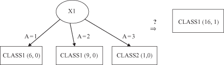
To analyze the possibility of replacing the subtree with a leaf node it is necessary to compute a predicted error PE for the initial tree and for a replaced node. Using default confidence of 25%, the upper confidence limits for all nodes are collected from statistical tables: U
25%
(6,0) = 0.206, U
25%
(9,0) = 0.143, U
25%
(1,0) = 0.750, and U
25%
(16,1) = 0.157. Using these values, the predicted errors for the initial tree and the replaced node are
