Data Mining (55 page)
Authors: Mehmed Kantardzic

CART uses the
Gini
diversity index as a splitting criterion instead of information-based criteria for C4.5. The CART authors favor the Gini criterion over information gain because the Gini can be extended to include symmetrized costs, and it is computed more rapidly than information gain. The Gini index is used to select the feature at each internal node of the decision tree. We define the Gini index for a data set
S
as follows:
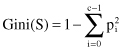
where
- c is the number of predefined classes,
- C
i
are classes for i = 1, … , c − 1, - s
i
is the number of samples belonging to class C
i
, and - p
i=
s
i
/S is a relative frequency of class C
i
in the set.
This metric indicates the partition purity of the data set
S
. For branch prediction where we have two classes the Gini index lies within [0, 0.5]. If all the data in
S
belong to the same class,
Gini S
equals the minimum value 0, which means that
S
is pure. If
Gini S
equals 0.5, all observations in
S
are equally distributed among two classes. This decreases as a split favoring one class: for instance a 70/30 distribution produces Gini index of 0.42. If we have more than two classes, the maximum possible value for index increases; for instance, the worst possible diversity for three classes is a 33% split, and it produces a
Gini
value of 0.67. The Gini coefficient, which ranges from 0 to 1 (for extremely large number of classes), is multiplied by 100 to range between 0 and 100 in some commercial tools.
The quality of a split on a feature into
k
subsets
S
i
is then computed as the weighted sum of the Gini indices of the resulting subsets:
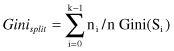
where
- n
i
is the number of samples in subset S
i
after splitting, and - n is the total number of samples in the given node.
Thus,
Gini
split
is calculated for all possible features, and the feature with minimum
Gini
split
is selected as split point. The procedure is repetitive as in C4.5. We may compare the results of CART and C4.5 attribute selection by applying entropy index (C4.5) and Gini index (CART) for splitting Attribute1 in Table
6.1
. While we already have results for C4.5 (gain ratio for Attribute 1), Gini
split
index for the same attribute may be calculated as:
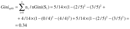
Interpretation of the absolute value for Gini
split
index is not important. It is important that relatively this value is lower for AttributeA1 than for the other two attributes in Table
6.1
. The reader may easily check this claim. Therefore, based on Gini index Attribute1 is selected for splitting. It is the same result obtained in C4.5 algorithm using an entropy criterion. Although the results are the same in this example, for many other data sets there could be (usually small) differences in results between these two approaches.
CART also supports the
twoing
splitting criterion, which can be used for multi-class problems. At each node, the classes are separated into two superclasses containing disjoint and mutually exhaustive classes. A splitting criterion for a two-class problem is used to find the attribute, and the two superclasses that optimize the two-class criterion. The approach gives “strategic” splits in the sense that several classes that are similar are grouped together. Although twoing splitting rule allows us to build more balanced trees, this algorithm works slower than Gini rule. For example, if the total number of classes is equal to K, then we will have 2K − 1 possible grouping into two classes. It can be seen that there is a small difference between trees constructed using Gini and trees constructed via twoing rule. The difference can be seen mainly at the bottom of the tree where the variables are less significant in comparison with the top of the tree.
Pruning technique used in CART is called minimal cost complexity pruning, while C4.5 uses binomial confidence limits. The proposed approach assumes that the bias in the re-substitution error of a tree increases linearly with the number of leaf nodes. The cost assigned to a subtree is the sum of two terms: the re-substitution error and the number of leaves times a complexity parameter α. It can be shown that, for every α value, there exists a unique smallest tree minimizing cost of the tree. Note that, although α runs through a continuum of values, there are at most a finite number of possible subtrees for analysis and pruning.
Unlike C4.5, CART does not penalize the splitting criterion during the tree construction if examples have unknown values for the attribute used in the split. The criterion uses only those instances for which the value is known. CART finds several surrogate splits that can be used instead of the original split. During classification, the first surrogate split based on a known attribute value is used. The surrogates cannot be chosen based on the original splitting criterion because the subtree at each node is constructed based on the original split selected. The surrogate splits are therefore chosen to maximize a measure of predictive association with the original split. This procedure works well if there are attributes that are highly correlated with the chosen attribute.
As its name implies, CART also supports building regression trees. Regression trees are somewhat simpler than classification trees because the growing and pruning criteria used in CART are the same. The regression tree structure is similar to a classification tree, except that each leaf predicts a real number. The re-substitution estimate for pruning the tree is the mean-squared error.
Among the main advantages of CART method is its robustness to outliers and noisy data. Usually the splitting algorithm will isolate outliers in an individual node or nodes. Also, an important practical property of CART is that the structure of its classification or regression trees is invariant with respect to monotone transformations of independent variables. One can replace any variable with its logarithm or square root value, the structure of the tree will not change. One of the disadvantages of CART is that the system may have unstable decision trees. Insignificant modifications of learning samples, such as eliminating several observations, could lead to radical changes in a decision tree: with a significant increase or decrease in tree complexity are changes in splitting variables and values.
C4.5 and CART are two popular algorithms for decision tree induction; however, their corresponding splitting criteria, information gain, and Gini index are considered to be skew-sensitive. In other words, they are not applicable, or at least not successfully applied, in cases where classes are not equally distributed in training and testing data sets. It becomes important to design a decision tree-splitting criterion that captures the divergence in distributions without being dominated by the class priors. One of the proposed solutions is the
Hellinger distance
as a decision tree-splitting criterion. Recent experimental results show that this distance measure is skew-insensitive.
For application as a decision tree-splitting criterion, we assume a countable space, so all continuous features are discretized into p partitions or bins. Assuming a two-class problem (class+ and class−), let X+ be samples belonging to class+, and X− are samples with class−. Then, we are essentially interested in calculating the “distance” in the normalized frequencies distributions aggregated over all the partitions of the two-class distributions X+ and X−. The Hellinger distance between X+ and X− is:
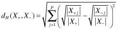
This formulation is strongly skew-insensitive. Experiments with real-world data show that the proposed measure may be successfully applied to cases where X+ X−. It essentially captures the divergence between the feature value distributions given the two different classes.
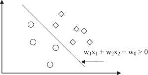
Recent developments in the field extend technology toward multivariate trees. In a multivariate tree, at a decision node, all input dimensions can be used for testing (e.g., w
1
x
1
+ w
2
x
2
+ w
0
> 0 as presented in Fig.
6.12
). It is a hyperplane with an arbitrary orientation. This is 2
d
(
N
d
) possible hyperplanes and exhaustive search is not practical.
Figure 6.12.
Multivariate decision node.