Data Mining (51 page)
Authors: Mehmed Kantardzic

and corresponding gain is

Based on the gain criterion, the decision-tree algorithm will select test x
1
as an initial test for splitting the database T because this gain is higher. To find the optimal test it will be necessary to analyze a test on Attribute2, which is a numeric feature with continuous values. In general, C4.5 contains mechanisms for proposing three types of tests:
1.
The “standard” test on a discrete attribute, with one outcome and one branch for each possible value of that attribute (in our example these are both tests x
1
for Attribute1 and x
2
for Attribute3).
2.
If attribute Y has continuous numeric values, a binary test with outcomes Y ≤ Z and Y > Z could be defined by comparing its value against a threshold value Z.
3.
A more complex test is also based on a discrete attribute, in which the possible values are allocated to a variable number of groups with one outcome and branch for each group.
While we have already explained standard test for categorical attributes, additional explanations are necessary about a procedure for establishing tests on attributes with numeric values. It might seem that tests on continuous attributes would be difficult to formulate, since they contain an arbitrary threshold for splitting all values into two intervals. But there is an algorithm for the computation of optimal threshold value Z. The training samples are first sorted on the values of the attribute Y being considered. There are only a finite number of these values, so let us denote them in sorted order as {v
1
, v
2
, … , v
m
}. Any threshold value lying between v
i
and v
i+1
will have the same effect as dividing the cases into those whose value of the attribute Y lies in {v
1
, v
2
, … , v
i
} and those whose value is in {v
i+1
, v
i+2
, … , v
m
}. There are thus only m-1 possible splits on Y, all of which should be examined systematically to obtain an optimal split. It is usual to choose the midpoint of each interval, (v
i
+ v
i+1
)/2, as the representative threshold. The algorithm C4.5 differs in choosing as the threshold a smaller value v
i
for every interval {v
i
, v
i+1
}, rather than the midpoint itself. This ensures that the threshold values appearing in either the final decision tree or rules or both actually occur in the database.
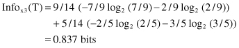
To illustrate this threshold-finding process, we could analyze, for our example of database T, the possibilities of Attribute2 splitting. After a sorting process, the set of values for Attribute2 is {65, 70, 75, 78, 80, 85, 90, 95, 96} and the set of potential threshold values Z is {65, 70, 75, 78, 80, 85, 90, 95}. Out of these eight values the optimal Z (with the highest information gain) should be selected. For our example, the optimal Z value is Z = 80 and the corresponding process of information-gain computation for the test x
3
(Attribute2 ≤ 80 or Attribute2 > 80) is the following:

Now, if we compare the information gain for the three attributes in our example, we can see that Attribute1 still gives the highest gain of 0.246 bits and therefore this attribute will be selected for the first splitting in the construction of a decision tree. The root node will have the test for the values of Attribute1, and three branches will be created, one for each of the attribute values. This initial tree with the corresponding subsets of samples in the children nodes is represented in Figure
6.4
.
Figure 6.4.
Initial decision tree and subset cases for a database in Table
6.1
.
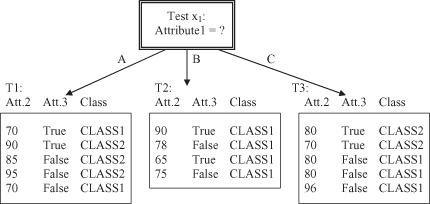
After initial splitting, every child node has several samples from the database, and the entire process of test selection and optimization will be repeated for every child node. Because the child node for test x
1
, Attribute1 = B, has four cases and all of them are in CLASS1, this node will be the leaf node, and no additional tests are necessary for this branch of the tree.
For the remaining child node where we have five cases in subset T
1
, tests on the remaining attributes can be performed; an optimal test (with maximum information gain) will be test x
4
with two alternatives: Attribute2 ≤ 70 or Attribute2 > 70.

Using Attribute2 to divide T
1
into two subsets (test x
4
represents the selection of one of two intervals), the resulting information is given by:
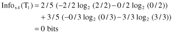
The information gained by this test is maximal:
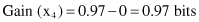
and two branches will create the final leaf nodes because the subsets of cases in each of the branches belong to the same class.
A similar computation will be carried out for the third child of the root node. For the subset T
3
of the database T, the selected optimal test x
5
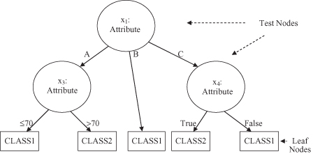
is the test on Attribute3 values. Branches of the tree, Attribute3 = True and Attribute3 = False, will create uniform subsets of cases that belong to the same class. The final decision tree for database T is represented in Figure
6.5
.
Figure 6.5.
A final decision tree for database T given in Table
6.1
.
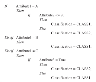
Alternatively, a decision tree can be presented in the form of an executable code (or pseudo-code) with if-then constructions for branching into a tree structure. The transformation of a decision tree from one representation to the other is very simple and straightforward. The final decision tree for our example is given in pseudocode in Figure
6.6
.
Figure 6.6.
A decision tree in the form of pseudocode for the database T given in Table
6.1
.