Data Mining (24 page)
Authors: Mehmed Kantardzic

(a)
Rank the features using a comparison of means and variances.
(b)
Rank the features using Relief algorithm. Use all samples for the algorithm (m = 7).
4.
Given four-dimensional samples where the first two dimensions are numeric and the last two are categorical
(a)
Apply a method for unsupervised feature selection based on entropy measure to reduce one dimension from the given data set.
(b)
Apply Relief algorithm under the assumption that X4 is output (classification) feature.
5.
(a)
Perform bin-based value reduction with the best cutoffs for the following:
(i)
the feature I
3
in problem 3 using mean values as representatives for two bins.
(ii)
the feature X
2
in problem 4 using the closest boundaries for two bin representatives.
(b)
Discuss the possibility of applying approximation by rounding to reduce the values of numeric attributes in problems 3 and 4.
6.
Apply the ChiMerge technique to reduce the number of values for numeric attributes in problem 3.
Reduce the number of numeric values for feature I
1
and find the final, reduced number of intervals.
Reduce the number of numeric values for feature I
2
and find the final, reduced number of intervals.
Reduce the number of numeric values for feature I
3
and find the final, reduced number of intervals.
Discuss the results and benefits of dimensionality reduction obtained in (a), (b), and (c).
7.
Explain the differences between averaged and voted combined solutions when random samples are used to reduce dimensionality of a large data set.
8.
How can the incremental-sample approach and the average-sample approach be combined to reduce cases in large data sets.
9.
Develop a software tool for feature ranking based on means and variances. Input data set is represented in the form of flat file with several features.
10.
Develop a software tool for ranking features using entropy measure. The input data set is represented in the form of a flat file with several features.
11.
Implement the ChiMerge algorithm for automated discretization of selected features in a flat input file.
12.
Given the data set F = {4, 2, 1, 6, 4, 3, 1, 7, 2, 2}, apply two iterations of
bin method for values reduction
with best cutoffs. Initial number of bins is 3. What are the final medians of bins, and what is the total minimized error?
13.
Assume you have 100 values that are all different, and use equal width discretization with 10 bins.
(a)
What is the largest number of records that could appear in one bin?
(b)
What is the smallest number of records that could appear in one bin?
(c)
If you use equal height discretization with 10 bins, what is largest number of records that can appear in one bin?
(d)
If you use equal height discretization with 10 bins, what is smallest number of records that can appear in one bin?
(e)
Now assume that the maximum value frequency is 20. What is the largest number of records that could appear in one bin with equal width discretization (10 bins)?
(f)
What about with equal height discretization (10 bins)?
3.10 REFERENCES FOR FURTHER STUDY
Fodor, I. K., A Survey of Dimension Reduction Techniques,
LLNL Technical Report
, June 2002.
The author reviews PCA and FA, respectively, the two most widely used linear dimension-reduction methods based on second-order statistics. However, many data sets of interest are not realizations from Gaussian distributions. For those cases, higher order dimension-reduction methods, using information not contained in the covariance matrix, are more appropriate. It includes ICA and method of random projections.
Liu, H., H. Motoda, eds.,
Instance Selection and Construction for Data Mining
, Kluwer Academic Publishers, Boston, MA, 2001.
Many different approaches have been used to address the data-explosion issue, such as algorithm scale-up and data reduction. Instance, sample, or tuple selection pertains to methods that select or search for a representative portion of data that can fulfill a data-mining task as if the whole data were used. This book brings researchers and practitioners together to report new developments and applications in instance-selection techniques, to share hard-learned experiences in order to avoid similar pitfalls, and to shed light on future development.
Liu, H., H. Motoda,
Feature Selection for Knowledge Discovery and Data Mining
, (Second Printing), Kluwer Academic Publishers, Boston, MA, 2000.
The book offers an overview of feature-selection methods and provides a general framework in order to examine these methods and categorize them. The book uses simple examples to show the essence of methods and suggests guidelines for using different methods under various circumstances.
Liu, H., H. Motoda,
Computational Methods of Feature Selection
, CRC Press, Boston, MA, 2007.
The book represents an excellent surveys, practical guidance, and comprehensive tutorials from leading experts. It paints a picture of the state-of-the-art techniques that can boost the capabilities of many existing data-mining tools and gives the novel developments of feature selection that have emerged in recent years, including causal feature selection and Relief. The book contains real-world case studies from a variety of areas, including text classification, web mining, and bioinformatics.
Saul, L. K., et al., Spectral Methods for Dimensionality Reduction, in
Semisupervised Learning
, B. Schööelkopf, O. Chapelle and A. Zien eds., MIT Press, Cambridge, MA, 2005.
Spectral methods have recently emerged as a powerful tool for nonlinear dimensionality reduction and manifold learning. These methods are able to reveal low-dimensional structure in high-dimensional data from the top or bottom eigenvectors of specially constructed matrices. To analyze data that lie on a low-dimensional sub-manifold, the matrices are constructed from sparse weighted graphs whose vertices represent input patterns and whose edges indicate neighborhood relations.
Van der Maaten, L. J. P., E. O. Postma, H. J. Van den Herik, Dimensionality Reduction: A Comparative Review,
Citeseer
, Vol. 10, February 2007, pp. 1–41.
http://www.cse.wustl.edu/~mgeotg/readPapers/manifold/maaten2007_survey.pdf
In recent years, a variety of nonlinear dimensionality-reduction techniques have been proposed that aim to address the limitations of traditional techniques such as PCA. The paper presents a review and systematic comparison of these techniques. The performances of the nonlinear techniques are investigated on artificial and natural tasks. The results of the experiments reveal that nonlinear techniques perform well on selected artificial tasks, but do not outperform the traditional PCA on real-world tasks. The paper explains these results by identifying weaknesses of current nonlinear techniques, and suggests how the performance of nonlinear dimensionality-reduction techniques may be improved.
Weiss, S. M., N. Indurkhya,
Predictive Data Mining: A Practical Guide
, Morgan Kaufman, San Francisco, CA, 1998.
This book focuses on the data-preprocessing phase in successful data-mining applications. Preparation and organization of data and development of an overall strategy for data mining are not only time-consuming processes but fundamental requirements in real-world data mining. A simple presentation of topics with a large number of examples is an additional strength of the book.
4
LEARNING FROM DATA
Chapter Objectives
- Analyze the general model of inductive learning in observational environments.
- Explain how the learning machine selects an approximating function from the set of functions it supports.
- Introduce the concepts of risk functional for regression and classification problems.
- Identify the basic concepts in statistical learning theory (SLT) and discuss the differences between inductive principles, empirical risk minimization (ERM), and structural risk minimization (SRM).
- Discuss the practical aspects of the Vapnik-Chervonenkis (VC) dimension concept as an optimal structure for inductive-learning tasks.
- Compare different inductive-learning tasks using graphical interpretation of approximating functions in a two-dimensional (2-D) space.
- Explain the basic principles of support vector machines (SVMs).
- Specify K nearest neighbor classifier: algorithm and applications.
- Introduce methods for validation of inductive-learning results.
Many recent approaches to developing models from data have been inspired by the learning capabilities of biological systems and, in particular, those of humans. In fact, biological systems learn to cope with the unknown, statistical nature of the environment in a data-driven fashion. Babies are not aware of the laws of mechanics when they learn how to walk, and most adults drive a car without knowledge of the underlying laws of physics. Humans as well as animals also have superior pattern-recognition capabilities for such tasks as identifying faces, voices, or smells. People are not born with such capabilities, but learn them through data-driven interaction with the environment.
It is possible to relate the problem of learning from data samples to the general notion of inference in classical philosophy. Every predictive-learning process consists of two main phases:
1.
learning or estimating unknown dependencies in the system from a given set of samples, and
2.
using estimated dependencies to predict new outputs for future input values of the system.
These two steps correspond to the two classical types of inference known as
induction
(progressing from particular cases—training data—to a general dependency or model) and
deduction
(progressing from a general model and given input values to particular cases of output values). These two phases are shown graphically in Figure
4.1
.
Figure 4.1.
Types of inference: induction, deduction, and transduction.
A unique estimated model implies that a learned function can be applied everywhere, that is, for all possible input values. Such global-function estimation can be overkill, because many practical problems require one to deduce estimated outputs only for a few given input values. In that case, a better approach may be to estimate the outputs of the unknown function for several points of interest directly from the training data without building a global model. Such an approach is called
transductive
inference in which a local estimation is more important than a global one. An important application of the
transductive
approach is a process of mining association rules, which is described in detail in Chapter 8. It is very important to mention that the standard formalization of machine learning does not apply to this type of inference.
The process of inductive learning and estimating the model may be described, formalized, and implemented using different learning methods. A learning method is an algorithm (usually implemented in software) that estimates an unknown mapping (dependency) between a system’s inputs and outputs from the available data set, namely, from known samples. Once such a dependency has been accurately estimated, it can be used to predict the future outputs of the system from the known input values. Learning from data has been traditionally explored in such diverse fields as statistics, engineering, and computer science. Formalization of the learning process and a precise, mathematically correct description of different inductive-learning methods were the primary tasks of disciplines such as SLT and artificial intelligence. In this chapter, we will introduce the basics of these theoretical fundamentals for inductive learning.
4.1 LEARNING MACHINE
Machine learning, as a combination of artificial intelligence and statistics, has proven to be a fruitful area of research, spawning a number of different problems and algorithms for their solution. These algorithms vary in their goals, in the available training data sets, and in the learning strategies and representation of data. All of these algorithms, however, learn by searching through an n-dimensional space of a given data set to find an acceptable generalization. One of the most fundamental machine-learning tasks is
inductive machine learning
where a generalization is obtained from a set of samples, and it is formalized using different techniques and models.
We can define inductive learning as the process of estimating an unknown input–output dependency or structure of a system, using limited number of observations or measurements of inputs and outputs of the system. In the theory of inductive learning, all data in a learning process are organized, and each instance of input–output pairs we use a simple term known as a sample. The general learning scenario involves three components, represented in Figure
4.2
.
1.
a generator of random input vectors X,
2.
a system that returns an output Y for a given input vector X, and
3.
a learning machine that estimates an unknown (input X, output Y″) mapping of the system from the observed (input X, output Y) samples.
Figure 4.2.
A learning machine uses observations of the system to form an approximation of its output.
This formulation is very general and describes many practical, inductive-learning problems such as interpolation, regression, classification, clustering, and density estimation. The generator produces a random vector X, which is drawn independently from any distribution. In statistical terminology, this situation is called an observational setting. It differs from the designed-experiment setting, which involves creating a deterministic sampling scheme, optimal for a specific analysis according to experimental design theory. The learning machine has no control over which input values were supplied to the system, and therefore, we are talking about an observational approach in inductive machine-learning systems.
The second component of the inductive-learning model is the system that produces an output value Y for every input vector X according to the conditional probability p(Y/X), which is unknown. Note that this description includes the specific case of a deterministic system where Y = f(X). Real-world systems rarely have truly random outputs; however, they often have unmeasured inputs. Statistically, the effects of these unobserved inputs on the output of the system can be characterized as random and represented with a probability distribution.
An inductive-learning machine tries to form generalizations from particular, true facts, which we call the training data set. These generalizations are formalized as a set of functions that approximate a system’s behavior. This is an inherently difficult problem, and its solution requires a priori knowledge in addition to data. All inductive-learning methods use a priori knowledge in the form of the selected class of approximating functions of a learning machine. In the most general case, the learning machine is capable of implementing a set of functions f(X, w), w ∈ W, where X is an input, w is a parameter of the function, and W is a set of abstract parameters used only to index the set of functions. In this formulation, the set of functions implemented by the learning machine can be any set of functions. Ideally, the choice of a set of approximating functions reflects a priori knowledge about the system and its unknown dependencies. However, in practice, because of the complex and often informal nature of a priori knowledge, specifying such approximating functions may be, in many cases, difficult or impossible.
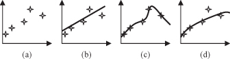
To explain the selection of approximating functions, we can use a graphical interpretation of the inductive-learning process. The task of inductive inference is this: Given a collection of samples (xi, f[xi]), return a function h(x) that approximates f(x). The function h(x) is often called a hypothesis. Figure
4.3
shows a simple example of this task, where the points in 2-D are given in Figure
4.3
a, and it is necessary to find “the best” function through these points. The true f(x) is unknown, so there are many choices for h(x). Without more knowledge, we have no way of knowing which one to prefer among three suggested solutions (Fig.
4.3
b,c,d). Because there are almost always a large number of possible, consistent hypotheses, all learning algorithms search through the solution space based on given criteria. For example, the criterion may be a linear approximating function that has a minimum distance from all given data points. This a priori knowledge will restrict the search space to the functions in the form given in Figure
4.3
b.
Figure 4.3.
Three hypotheses for a given data set.
There is also an important distinction between the two types of approximating functions we usually use in an inductive-learning process. Their parameters could be
linear or nonlinear.
Note that the notion of linearity is with respect to parameters rather than input variables. For example, polynomial regression in the form
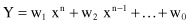
is a linear method, because the parameters w
i
in the function are linear (even if the function by itself is nonlinear). We will see later that some learning methods such as multilayer, artificial, neural networks provide an example of nonlinear parametrization, since the output of an approximating function depends nonlinearly on parameters. A typical factor in these functions is e
−ax
, where a is a parameter and x is the input value. Selecting the approximating functions f(X, w) and estimating the values of parameters w are typical steps for every inductive-learning method.