Data Mining (22 page)
Authors: Mehmed Kantardzic

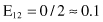
If either R
i
or C
j
in the contingency table is 0, E
ij
is set to a small value, for example, E
ij
= 0.1. The reason for this modification is to avoid very small values in the denominator of the test. The degree of freedom parameter of the χ
2
test is for one less than the number of classes. When more than one feature has to be discretized, a threshold for the maximum number of intervals and a confidence interval for the χ
2
test should be defined separately for each feature. If the number of intervals exceeds the maximum, the algorithm ChiMerge may continue with a new, reduced value for confidence.
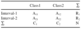
For a classification problem with two classes (k = 2), where the merging of two intervals is analyzed, the contingency table for 2 × 2 has the form given in Table
3.5
. A
11
represents the number of samples in the first interval belonging to the first class; A
12
is the number of samples in the first interval belonging to the second class; A
21
is the number of samples in the second interval belonging to the first class; and finally A
22
is the number of samples in the second interval belonging to the second class.
TABLE 3.5.
A Contingency Table for 2 × 2 Categorical Data
We will analyze the ChiMerge algorithm using one relatively simple example, where the database consists of 12 two-dimensional samples with only one continuous feature (F) and an output classification feature (K). The two values, 1 and 2, for the feature K represent the two classes to which the samples belong. The initial data set, already sorted with respect to the continuous numeric feature F, is given in Table
3.6
.
TABLE 3.6.
Data on the Sorted Continuous Feature F with Corresponding Classes K
| Sample | F | K |
| 1 | 1 | 1 |
| 2 | 3 | 2 |
| 3 | 7 | 1 |
| 4 | 8 | 1 |
| 5 | 9 | 1 |
| 6 | 11 | 2 |
| 7 | 23 | 2 |
| 8 | 37 | 1 |
| 9 | 39 | 2 |
| 10 | 45 | 1 |
| 11 | 46 | 1 |
| 12 | 59 | 1 |
We can start the algorithm of a discretization by selecting the smallest χ
2
value for intervals on our sorted scale for F. We define a middle value in the given data as a splitting interval point. For our example, interval points for feature F are 0, 2, 5, 7.5, 8.5, and 10. Based on this distribution of intervals, we analyze all adjacent intervals trying to find a minimum for the χ
2
test. In our example, χ
2
was the minimum for intervals [7.5, 8.5] and [8.5, 10]. Both intervals contain only one sample, and they belong to class K = 1. The initial contingency table is given in Table
3.7
.
TABLE 3.7.
Contingency Table for Intervals [7.5, 8.5] and [8.5, 10]
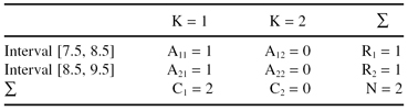
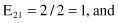
Based on the values given in the table, we can calculate the expected values

and the corresponding χ
2
test

For the degree of freedom d = 1, and χ
2
= 0.2 < 2.706 (the threshold value from the tables for chi-squared distribution for α = 0.1), we can conclude that there are no significant differences in relative class frequencies and that the selected intervals can be merged. The merging process will be applied in one iteration only for two adjacent intervals with a minimum χ
2
and, at the same time, with χ
2
< threshold value. The iterative process will continue with the next two adjacent intervals that have the minimum χ
2
. We will just show one additional step, somewhere in the middle of the merging process, where the intervals [0, 7.5] and [7.5, 10] are analyzed. The contingency table is given in Table
3.8
, and expected values are