Data Mining (17 page)
Authors: Mehmed Kantardzic

where W
k×p
is the linear transformation weight matrix. Such linear techniques are simpler and easier to implement than more recent methods considering nonlinear transforms.
In general, the process reduces feature dimensions by combining features instead of by deleting them. It results in a new set of fewer features with totally new values. One well-known approach is merging features by
principal components
. The features are examined collectively, merged, and transformed into a new set of features that, it is hoped, will retain the original information content in a reduced form. The basic transformation is linear. Given p features, they can be transformed into a single new feature F′ by the simple application of weights:
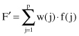
Most likely, a single set of weights, w(j), will not be an adequate transformation for a complex multidimensional data set, and up to p transformations are generated. Each vector of p features combined by weights w is called a principal component, and it defines a new transformed feature. The first vector of m weights is expected to be the strongest, and the remaining vectors are ranked according to their expected usefulness in reconstructing the original data. Eliminating the bottom-ranked transformation will reduce dimensions. The complexity of computation increases significantly with the number of features. The main weakness of the method is that it makes an advance assumption to a linear model that maximizes the variance of features. Formalization of PCA and the basic steps of the corresponding algorithm for selecting features are given in Section 3.4.
Examples of additional methodologies in feature extraction include factor analysis (FA), independent component analysis (ICA), and multidimensional scaling (MDS). Probably the last one is the most popular and it represents the basis for some new, recently developed techniques. Given n samples in a p-dimensional space and an n × n matrix of distances measures among the samples, MDS produces a k-dimensional (k p) representation of the items such that the distances among the points in the new space reflect the distances in the original data. A variety of distance measures may be used in the technique and the main characteristics for all these measures is: The more similar two samples are, the smaller their distance is. Popular distance measures include the Euclidean distance (L2 norm), the Manhattan distance (L1, absolute norm), and the maximum norm; more details about these measures and their applications are given in Chapter 9. MDS has been typically used to transform the data into two or three dimensions; visualizing the result to uncover hidden structure in the data. A rule of thumb to determine the maximum number of k is to ensure that there are at least twice as many pairs of samples than the number of parameters to be estimated, resulting in p ≥ k + 1. Results of the MDS technique are indeterminate with respect to translation, rotation, and reflection of data.
PCA and metric MDS are both simple methods for linear dimensionality reduction, where an alternative to MDS is FastMap, a computationally efficient algorithm. The other variant,
Isomap
, has recently emerged as a powerful technique for nonlinear dimensionality reduction and is primarily a graph-based method.
Isomap
is based on computing the low-dimensional representation of a high-dimensional data set that most faithfully preserves the pairwise distances between input samples as measured along geodesic distance (details about geodesic are given in Chapter 12, the section about graph mining). The algorithm can be understood as a variant of MDS in which estimates of geodesic distances are substituted for standard Euclidean distances.
The algorithm has three steps. The first step is to compute the k-nearest neighbors of each input sample, and to construct a graph whose vertices represent input samples and whose (undirected) edges connect k-nearest neighbors. The edges are then assigned weights based on the Euclidean distance between nearest neighbors. The second step is to compute the pairwise distances between all nodes (i, j) along shortest paths through the graph. This can be done using the well-known Djikstra’s algorithm with complexity
O
(
n
2
log
n
+
n
2
k
). Finally, in the third step, the pairwise distances are fed as input to MDS to determine a new reduced set of features.
With the amount of data growing larger and larger, all feature-selection (and reduction) methods also face a problem of oversized data because of computers’ limited resources. But do we really need so much data for selecting features as an initial process in data mining? Or can we settle for less data? We know that some portion of a huge data set can represent it reasonably well. The point is which portion and how large should it be. Instead of looking for the right portion, we can randomly select a part, P, of a data set, use that portion to find the subset of features that satisfy the evaluation criteria, and test this subset on a different part of the data. The results of this test will show whether the task has been successfully accomplished. If an inconsistency is found, we shall have to repeat the process with a slightly enlarged portion of the initial data set. What should be the initial size of the data subset P? Intuitively, we know that its size should not be too small or too large. A simple way to get out of this dilemma is to choose a percentage of data, say 10%. The right percentage can be determined experimentally.
What are the results of a feature-reduction process, and why do we need this process for every specific application? The purposes vary, depending upon the problem on hand, but, generally, we want
1.
to
improve performances
of the model-generation process and the resulting model itself (typical criteria are speed of learning, predictive accuracy, and simplicity of the model);
2.
to
reduce dimensionality
of the model without reduction of its quality through
(a)
elimination of irrelevant features,
(b)
detection and elimination of redundant data and features,
(c)
identification of highly correlated features, and
(d)
extraction of independent features that determine the model; and
3.
to help the user
visualize
alternative results, which have fewer dimensions, to improve decision making.
3.3 RELIEF ALGORITHM
Reliefis a feature weight-based algorithm for feature selection inspired by the so-called instance-based learning. It relies on relevance evaluation of each feature given in a training data set, where samples are labeled (classification problems). The main idea of Relief is to compute a ranking score for every feature indicating how well this feature separates neighboring samples. The authors of the Relief algorithm, Kira and Rendell, proved that the ranking score is large for relevant features and small for irrelevant ones.
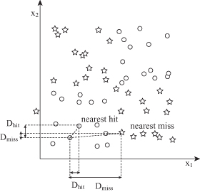
The core of the Relief algorithm is to estimate the quality of features according to how well their values distinguish between samples close to each other. Given training data S, the algorithm randomly selects subset of samples size m, where m is a user-defined parameter. Relief analyzes each feature based on a selected subset of samples. For each randomly selected sample X from a training data set, Relief searches for its two nearest neighbors: one from the same class, called nearest hit H, and the other one from a different class, called nearest miss M. An example for two-dimensional data is given in Figure
3.2
.
Figure 3.2.
Determining nearest hit H and nearest miss M samples.
The Relief algorithm updates the quality score W(A
i
) for all feature A
i
depending on the differences on their values for samples X, M, and H:

The process is repeated m times for randomly selected samples from the training data set and the scores W(A
i
) are accumulated for each sample. Finally, using threshold of relevancy τ, the algorithm detects those features that are statistically relevant to the target classification, and these are the features with W(A
i
) ≥ τ. We assume the scale of every feature is either nominal (including Boolean) or numerical (integer or real). The main steps of the Relief algorithm may be formalized as follows:
Initialize
: W(A
j
) = 0; i = 1, … , p (p is the number of features)
For i = 1 to m
Randomly select sample X from training data set S.
Find nearest hit H and nearest miss M samples.
For j = 1 to p

End.
End.
Output
: Subset of feature where W(A
j
) ≥ τ
For example, if the available training set is given in Table
3.2
with three features (the last one of them is classification decision) and four samples, the scoring values W for the features F
1
and F
2
may be calculated using Relief: