Data Mining (19 page)
Authors: Mehmed Kantardzic

The distribution of all similarities (distances) for a given data set is a characteristic of the organization and order of data in an n-dimensional space. This organization may be more or less ordered. Changes in the level of order in a data set are the main criteria for inclusion or exclusion of a feature from the feature set; these changes may be measured by entropy.
From information theory, we know that entropy is a global measure, and that it is less for ordered configurations and higher for disordered configurations. The proposed technique compares the entropy measure for a given data set before and after removal of a feature. If the two measures are close, then the reduced set of features will satisfactorily approximate the original set. For a data set of N samples, the entropy measure is
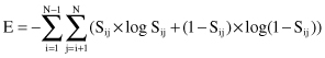
where S
ij
is the similarity between samples x
i
and x
j
. This measure is computed in each of the iterations as a basis for deciding the ranking of features. We rank features by gradually removing the least important feature in maintaining the order in the configurations of data. The steps of the algorithm are based on sequential backward ranking, and they have been successfully tested on several real-world applications.
1.
Start with the initial full set of feature F.
2.
For each feature f∈F, remove one feature f from F and obtain a subset F
f
. Find the difference between entropy for F and entropy for all F
f
. In the example in Figure
3.2
, we have to compare the differences (E
F
− E
F-F1
), (E
F
− E
F-F2
), and (E
F
− E
F-F3
).
3.
Let f
k
be a feature such that the difference between entropy for F and entropy for F
fk
is minimum.
4.
Update the set of feature F = F − {f
k
}, where “–” is a difference operation on sets. In our example, if the difference (E
F
− E
F-F1
) is minimum, then the reduced set of features is {F
2
, F
3
}. F
1
becomes the bottom of the ranked list.
5.
Repeat steps 2–4 until there is only one feature in F.
A ranking process may be stopped in any iteration, and may be transformed into a process of selecting features, using the additional criterion mentioned in step 4. This criterion is that the difference between entropy for F and entropy for F
f
should be less than the approved threshold value to reduce feature f
k
from set F. A computational complexity is the basic disadvantage of this algorithm, and its parallel implementation could overcome the problems of working with large data sets and large number of features sequentially.
3.5 PCA
The most popular statistical method for dimensionality reduction of a large data set is the Karhunen-Loeve (K-L) method, also called
PCA
. In various fields, it is also known as the singular value decomposition (SVD), the Hotelling transform, and the empirical orthogonal function (EOF) method. PCA is a method of transforming the initial data set represented by vector samples into a new set of vector samples with derived dimensions. The goal of this transformation is to concentrate the information about the differences between samples into a small number of dimensions. Practical applications confirmed that PCA is the best linear dimension-reduction technique in the mean-square error sense. Being based on the covariance matrix of the features, it is a second-order method. In essence, PCA seeks to reduce the dimension of the data by finding a few orthogonal linear combinations of the original features with the largest variance. Since the variance depends on the scale of the variables, it is customary to first standardize each variable to have mean 0 and standard deviation 1. After the standardization, the original variables with possibly different units of measurement are all in comparable units.
More formally, the basic idea can be described as follows: A set of n-dimensional vector samples X = {x
1
, x
2
, x
3
, … , x
m
} should be transformed into another set Y = {y
1
, y
2
, … , y
m
} of the same dimensionality, but y-s have the property that most of their information content is stored in the first few dimensions. This will allow us to reduce the data set to a smaller number of dimensions with low information loss.
The transformation is based on the assumption that high information corresponds to high variance. So, if we want to reduce a set of input dimensions X to a single dimension Y, we should transform X into Y as a matrix computation

choosing A such that Y has the largest variance possible for a given data set. The single dimension Y obtained in this transformation is called
the first principal component
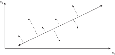
. The first principal component is an axis in the direction of maximum variance. It minimizes the distance of the sum of squares between data points and their projections on the component axis, as shown in Figure
3.4
where a two-dimensional space is transformed into a one-dimensional space in which the data set has the highest variance.
Figure 3.4.
The first principal component is an axis in the direction of maximum variance.
In practice, it is not possible to determine matrix A directly, and therefore we compute the covariance matrix S as a first step in feature transformation. Matrix S is defined as
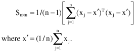
The eigenvalues of the covariance matrix S for the given data should be calculated in the next step. Finally, the m eigenvectors corresponding to the m largest eigenvalues of S define a linear transformation from the n-dimensional space to an m-dimensional space in which the features are uncorrelated. To specify the principal components we need the following additional explanations about the notation in matrix S:
1.
The eigenvalues of S
n×n
are λ
1
, λ
2
, … , λ
n
, where
2.
The eigenvectors e
1
, e
2
, … , e
n
correspond to eigenvalues λ
1
, λ
2
, … , λ
n
, and they are called the principal axes.
Principal axes are new, transformed axes of an n-dimensional space, where the new variables are uncorrelated, and variance for the
i
th component is equal to the
i
th eigenvalue. Because λ
i
’s are sorted, most of the information about the data set is concentrated in a few first-principal components. The fundamental question is how many of the principal components are needed to get a good representation of the data? In other words, what is the effective dimensionality of the data set? The easiest way to answer the question is to analyze the proportion of variance. Dividing the sum of the first m eigenvalues by the sum of all the variances (all eigenvalues), we will get the measure for the quality of representation based on the first m principal components. The result is expressed as a percentage, and if, for example, the projection accounts for over 90% of the total variance, it is considered to be good. More formally, we can express this ratio in the following way. The criterion for feature selection is based on the ratio of the sum of the
m
largest eigenvalues of S to the trace of S. That is a fraction of the variance retained in the m-dimensional space. If the eigenvalues are labeled so that λ
1
≥ λ
2
≥ … ≥ λ
n
, then the ratio can be written as
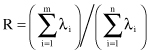
When the ratio R is sufficiently large (greater than the threshold value), all analyses of the subset of m features represent a good initial estimate of the n-dimensionality space. This method is computationally inexpensive, but it requires characterizing data with the covariance matrix S.
We will use one example from the literature to show the advantages of PCA. The initial data set is the well-known set of Iris data, available on the Internet for data-mining experimentation. This data set has four features, so every sample is a four-dimensional vector. The correlation matrix, calculated from the Iris data after normalization of all values, is given in Table
3.3
.