Data Mining (20 page)
Authors: Mehmed Kantardzic

TABLE 3.3.
The Correlation Matrix for Iris Data
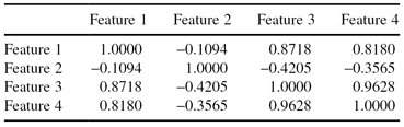
Based on the correlation matrix, it is a straightforward calculation of eigenvalues (in practice, usually, one of the standard statistical packages is used), and these final results for the Iris data are given in Table
3.4
.
TABLE 3.4.
The Eigenvalues for Iris Data
| Feature | Eigenvalue |
| Feature 1 | 2.91082 |
| Feature 2 | 0.92122 |
| Feature 3 | 0.14735 |
| Feature 4 | 0.02061 |
By setting a threshold value for R* = 0.95, we choose the first two features as the subset of features for further data-mining analysis, because

For the Iris data, the first two principal components should be adequate description of the characteristics of the data set. The third and fourth components have small eigenvalues and therefore, they contain very little variation; their influence on the information content of the data set is thus minimal. Additional analysis shows that based on the reduced set of features in the Iris data, the model has the same quality using different data-mining techniques (sometimes the results were even better than with the original features).
The interpretation of the principal components can be difficult at times. Although they are uncorrelated features constructed as linear combinations of the original features, and they have some desirable properties, they do not necessarily correspond to meaningful physical quantities. In some cases, such loss of interpretability is not satisfactory to the domain scientists, and they prefer others, usually feature-selection techniques.
3.6 VALUE REDUCTION
A reduction in the number of discrete values for a given feature is based on the second set of techniques in the data-reduction phase; these are the
feature-discretization techniques.
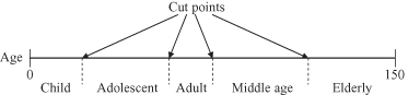
The task of feature-discretization techniques is to discretize the values of continuous features into a small number of intervals, where each interval is mapped to a discrete symbol. The benefits of these techniques are simplified data description and easy-to-understand data and final data-mining results. Also, more data-mining techniques are applicable with discrete feature values. An “old-fashioned” discretization is made manually, based on our a priori knowledge about the feature. For example, using common sense or consensus, a person’s age, given at the beginning of a data-mining process as a continuous value (between 0 and 150 years), may be classified into categorical segments: child, adolescent, adult, middle age, and elderly. Cutoff points are subjectively defined (Fig.
3.5
). Two main questions exist about this reduction process:
1.
What are the cutoff points?
2.
How does one select representatives of intervals?
Figure 3.5.
Discretization of the
age
feature.
Without any knowledge about a feature, a discretization is much more difficult and, in many cases, arbitrary. A reduction in feature values usually is not harmful for real-world data-mining applications, and it leads to a major decrease in computational complexity. Therefore, we will introduce, in the next two sections, several automated discretization techniques.
Within a column of a data set (set of feature values), the number of distinct values can be counted. If this number can be reduced, many data-mining methods, especially the logic-based methods explained in Chapter 6, will increase the quality of a data analysis. Reducing the number of values by smoothing feature values does not require a complex algorithm because each feature is smoothed independently of other features and the process is performed only once, without iterations.
Suppose that a feature has a range of numeric values, and that these values can be ordered from the smallest to the largest using standard greater-than and less-than operators. This leads naturally to the concept of
placing the values in bins
—partitioning into groups with close values. Typically, these bins have a close number of elements. All values in a bin will be merged into a single concept represented by a single value—usually either the mean or median of the bin’s values. The mean or the mode is effective for a moderate or large number of bins. When the number of bins is small, the closest boundaries of each bin can be candidates for representatives in a given bin.
For example, if a set of values for a given feature f is {3, 2, 1, 5, 4, 3, 1, 7, 5, 3}, then, after sorting, these values will be organized into an ordered set:
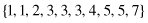
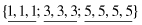
Now, it is possible to split the total set of values into three bins with a close number of elements in each bin:
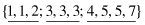

In the next step, different representatives can be selected for each bin. If the smoothing is performed based on bin modes, the new set of values for each bin will be
If the smoothing is performed based on mean values, then the new distribution for reduced set of values will be

