Data Mining (18 page)
Authors: Mehmed Kantardzic


TABLE 3.2.
Training Data Set for Applying
Relief
Algorithm
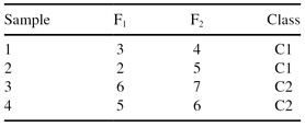
In this example the number of samples is low and therefore we use all samples (m = n) to estimate the feature scores. Based on the previous results feature F
1
is much more relevant in classification than feature F
2
. If we assign the threshold value of τ = 5, it is possible to eliminate feature F
2
and build the classification model only based on feature F
1
.
Relief is a simple algorithm that relies entirely on a statistical methodology. The algorithm employs few heuristics, and therefore it is efficient—its computational complexity is O(mpn). With m, number of randomly selected training samples, being a user-defined constant, the time complexity becomes O(pn), which makes it very scalable to data sets with both a huge number of samples
n
and a very high dimensionality p. When n is very large, it is assumed that m n. It is one of the few algorithms that can evaluate features for real-world problems with large feature space and large number of samples. Relief is also noise-tolerant and is unaffected by feature interaction, and this is especially important for hard data-mining applications. However, Relief does not help with removing redundant features. As long as features are deemed relevant to the class concept, they will be selected even though many of them are highly correlated to each other.
One of the Relief problems is to pick a proper value of τ. Theoretically, using the so-called Cebysev’s inequality τ may be estimated:

While the above formula determines τ in terms of α (data-mining model accuracy) and m (the training data set size), experiments show that the score levels display clear contrast between relevant and irrelevant features so τ can easily be determined by inspection.
Relief was extended to deal with multi-class problems, noise, redundant, and missing data. Recently, additional feature-selection methods based on feature weighting are proposed including ReliefF, Simba, and I-Relief, and they are improvements of the basic Relief algorithm.
3.4 ENTROPY MEASURE FOR RANKING FEATURES
A method for unsupervised feature selection or ranking based on entropy measure is a relatively simple technique, but with a large number of features its complexity increases significantly. The basic assumption is that all samples are given as vectors of a feature’s values without any classification of output samples. The approach is based on the observation that removing an irrelevant feature, a redundant feature, or both from a set may not change the basic characteristics of the data set. The idea is to remove as many features as possible and yet maintain the level of distinction between the samples in the data set as if no features had been removed. The algorithm is based on a similarity measure S that is in inverse proportion to the distance D between two n-dimensional samples. The distance measure D is small for close samples (close to 0) and large for distinct pairs (close to one). When the features are numeric, the similarity measure S of two samples can be defined as

where D
ij
is the distance between samples x
i
and x
j
and α is a parameter mathematically expressed as
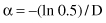
D is the average distance among samples in the data set. Hence, α is determined by the data. But, in a successfully implemented practical application, it was used a constant value of α = 0.5. Normalized Euclidean distance measure is used to calculate the distance D
ij
between two samples x
i
and x
j
:
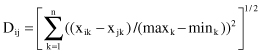
where n is the number of dimensions and max
k
and min
k
are maximum and minimum values used for normalization of the
k
th dimension.
All features are not numeric. The similarity for nominal variables is measured directly using Hamming distance:
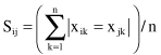
where |x
ik
= x
jk
| is 1 if x
ik
= x
jk
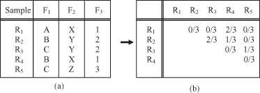
, and 0 otherwise. The total number of variables is equal to n. For mixed data, we can discretize numeric values and transform numeric features into nominal features before we apply this similarity measure. Figure
3.3
a is an example of a simple data set with three categorical features; corresponding similarities are given in Figure
3.3
b.
Figure 3.3.
A tabular representation of similarity measures S. (a) Data set with three features; (b) a table of similarity measures categorical feature S
ij
between samples.