Data Mining (27 page)
Authors: Mehmed Kantardzic

Summarizing SLT, in order to form a unique model of a system from finite data, any inductive-learning process requires the following:
1.
A wide, flexible set of
approximating functions
f(X, w), w ∈ W, that can be linear or nonlinear in parameters w.
2.
A priori knowledge (or assumptions) used to impose constraints on a potential solution. Usually such a priori knowledge orders the functions, explicitly or implicitly, according to some measure of their flexibility to fit the data. Ideally, the choice of a set of approximating functions reflects a priori knowledge about a system and its unknown dependencies.
3.
An inductive principle, or method of inference, specifying what has to be done. It is a general prescription for combining a priori knowledge with available training data in order to produce an estimate of an unknown dependency.
4.
A learning method, namely, a constructive, computational implementation of an inductive principle for a given class of approximating functions. There is a general belief that for learning methods with finite samples, the best performance is provided by a model of optimum complexity, which is selected based on the general principle known as Occam’s razor. According to this principle, we should seek simpler models over complex ones and optimize the model that is the trade-off between model complexity and the accuracy of fit to the training data.
4.3 TYPES OF LEARNING METHODS
There are two common types of the inductive-learning methods. They are known as
1.
supervised learning (or learning with a teacher), and
2.
unsupervised learning (or learning without a teacher).
Supervised learning
is used to estimate an unknown dependency from known input–output samples. Classification and regression are common tasks supported by this type of inductive learning. Supervised learning assumes the existence of a teacher—fitness function or some other external method of estimating the proposed model. The term “supervised” denotes that the output values for training samples are known (i.e., provided by a “teacher”).
Figure
4.8
a shows a block diagram that illustrates this form of learning. In conceptual terms, we may think of the teacher as having knowledge of the environment, with that knowledge being represented by a set of input–output examples. The environment with its characteristics and model is, however, unknown to the learning system. The parameters of the learning system are adjusted under the combined influence of the training samples and the error signal. The error signal is defined as the difference between the desired response and the actual response of the learning system. Knowledge of the environment available to the teacher is transferred to the learning system through the training samples, which adjust the parameters of the learning system. It is a closed-loop feedback system, but the unknown environment is not in the loop. As a performance measure for the system, we may think in terms of the mean-square error or the sum of squared errors over the training samples. This function may be visualized as a multidimensional error surface, with the free parameters of the learning system as coordinates. Any learning operation under supervision is represented as a movement of a point on the error surface. For the system to improve the performance over time and therefore learn from the teacher, the operating point on an error surface has to move down successively toward a minimum of the surface. The minimum point may be a local minimum or a global minimum. The basic characteristics of optimization methods such as stochastic approximation, iterative approach, and greedy optimization have been given in the previous section. An adequate set of input–output samples will move the operating point toward the minimum, and a supervised learning system will be able to perform such tasks as pattern classification and function approximation. Different techniques support this kind of learning, and some of them such as logistic regression, multilayered perceptron, and decision rules and trees will be explained in more detail in Chapters 5, 6, and 7.
Figure 4.8.
Two main types of inductive learning. (a) Supervised learning; (b) unsupervised learning.
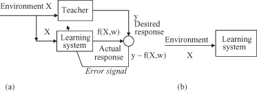
Under the unsupervised learning scheme, only samples with input values are given to a learning system, and there is no notion of the output during the learning process. Unsupervised learning eliminates the teacher and requires that the learner form and evaluate the model on its own. The goal of unsupervised learning is to discover “natural” structure in the input data. In biological systems, perception is a task learned via unsupervised techniques.
The simplified schema of unsupervised or self-organized learning, without an external teacher to oversee the learning process, is indicated in Figure
4.8
b. The emphasis in this learning process is on a task-independent measure of the quality of representation that is learned by the system. The free parameters w of the learning system are optimized with respect to that measure. Once the system has become tuned to the regularities of the input data, it develops the ability to form internal representations for encoding features of the input examples. This representation can be
global
, applicable to the entire input data set. These results are obtained with methodologies such as cluster analysis or some artificial neural networks, explained in Chapters 6 and 9. On the other hand, learned representation for some learning tasks can only be
local
, applicable to the specific subsets of data from the environment; association rules are a typical example of an appropriate methodology. It has been explained in more detail in Chapter 8.
4.4 COMMON LEARNING TASKS
The generic inductive-learning problem can be subdivided into several common learning tasks. The fundamentals of inductive learning, along with the classification of common learning tasks, have already been given in the introductory chapter of this book. Here, we would like to analyze these tasks in detail, keeping in mind that for each of these tasks, the nature of the loss function and the output differ. However, the goal of minimizing the risk based on training data is common to all tasks. We believe that visualization of these tasks will give the reader the best feeling about the complexity of the learning problem and the techniques required for its solution.
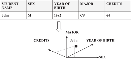
To obtain a graphical interpretation of the learning tasks, we start with the formalization and representation of data samples that are the “infrastructure” of the learning process. Every sample used in data mining represents one entity described with several attribute–value pairs. That is, one row in a tabular representation of a training data set, and it can be visualized as a point in an n-dimensional space, where n is the number of attributes (dimensions) for a given sample. This graphical interpretation of samples is illustrated in Figure
4.9
, where a student with the name John represents a point in a 4-D space that has four additional attributes.
Figure 4.9.
Data samples = points in an n-dimensional space.
When we have a basic idea of the representation of each sample, the training data set can be interpreted as a set of points in the n-dimensional space. Visualization of data and a learning process is difficult for large number of dimensions. Therefore, we will explain and illustrate the common learning tasks in a 2-D space, supposing that the basic principles are the same for a higher number of dimensions. Of course, this approach is an important simplification that we have to take care of, especially keeping in mind all the characteristics of large, multidimensional data sets, explained earlier under the topic “the curse of dimensionality.”
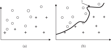
Let us start with the first and most common task in inductive learning:
classification
. This is a learning function that classifies a data item into one of several predefined classes. The initial training data set is given in Figure
4.10
a. Samples belong to different classes and therefore we use different graphical symbols to visualize each class. The final result of classification in a 2-D space is the curve shown in Figure
4.10
b, which best separates samples into two classes. Using this function, every new sample, even without a known output (the class to which it belongs), may be classified correctly. Similarly, when the problem is specified with more than two classes, more complex functions are a result of a classification process. For an n-dimensional space of samples the complexity of the solution increases exponentially, and the classification function is represented in the form of hypersurfaces in the given space.
Figure 4.10.
Graphical interpretation of classification. (a) Training data set; (b) classification function.
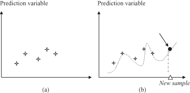
The second learning task is
regression
.The result of the learning process in this case is a learning function, which maps a data item to a real-value prediction variable. The initial training data set is given in Figure
4.11
a. The regression function in Figure
4.11
b was generated based on some predefined criteria built inside a data-mining technique. Based on this function, it is possible to estimate the value of a prediction variable for each new sample. If the regression process is performed in the time domain, specific subtypes of data and inductive-learning techniques can be defined.
Figure 4.11.
Graphical interpretation of regression. (a) Training data set; (b) regression function.
Clustering
is the most common unsupervised learning task. It is a descriptive task in which one seeks to identify a finite set of categories or clusters to describe the data. Figure
4.12
a shows the initial data, and they are grouped into clusters, as shown in Figure
4.12
b, using one of the standard distance measures for samples as points in an n-dimensional space. All clusters are described with some general characteristics, and the final solutions differ for different clustering techniques. Based on results of the clustering process, each new sample may be assigned to one of the previously found clusters, using its similarity with the cluster characteristics of the sample as a criterion.