Data Mining (30 page)
Authors: Mehmed Kantardzic

and representing scalar product of vectors by definition,

we obtain

where || || represents Euclidean normor

Therefore, the problem of “maximum margin” is represented as a maximum of a distance parameter d, which is a function of parameters w. Maximizing d means maximizing 1/|w| or minimizing |w|. The learning problem may be reformulated as:

subject to the constraints of linear separability. So, the final problem for optimization is

The problem of optimization under constraints may be transformed using the Lagrangian
L
(
w
,
b
)

where α
i
are the Lagrange multipliers, one for each data point. The first term is the same as the original objective function, and the second term captures the inequality constraints. The Lagrangian has to be minimized with respect to
w
and
b
:

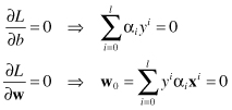
Substituting results of partial derivatives into
L
lead to the dual formulation of the optimization problem that has to be maximized with respect to the constraints α
i
≥ 0.

The dual Lagrangian D(α) involves only the Lagrangian multipliers α
i
and the training data (there is no more parameters w and b). Finding the solution for real-world problems will usually require application of quadratic programming (QP) optimization techniques. This problem has a global optimum. The optimization approach for SVM provides an accurate implementation of the SRM inductive principle. When α
i
parameters are determined, it is necessary to determine the values for w and b and they determine final classification hyperplane. It is important to note that dual function D is a function of only scalar products of sample vectors, not of vectors alone. Once the solution has been found in the form of a vector the optimal separating hyperplane is given by

where x
r
and x
s
are any support vectors (SVs) from each class. The classifier can then be constructed as:

Only the points x
i
, which will have nonzero Lagrangian multipliers α
0
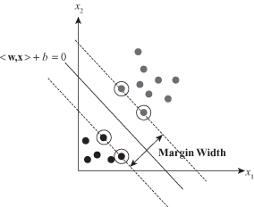
, are termed SVs. If the data are linearly separable, all the SVs will lie on the margin and hence the number of SVs can be very small as it is represented in Figure
4.21
. This “sparse” representation can be viewed as data compression in the construction of the classifier. The SVs are the “hard” cases; these are the training samples that are most difficult to classify correctly and that lie closest to the decision boundary.
Figure 4.21.
A maximal margin hyperplane with its support vectors encircled.
