Data Mining (32 page)
Authors: Mehmed Kantardzic

The polynomial kernel is valid for all positive integers d ≥ 1. The Gaussian kernel is one of a group of kernel functions known as radial basis functions (RBFs). RBFs are kernel functions that depend only on the geometric distance between x and y, and the kernel is valid for all nonzero values of the kernel width
σ
. It is probably the most useful and commonly applied kernel function. The concept of a kernel mapping function is very powerful, such as in the example given in Figure
4.25
. It allows SVM models to perform separations even with very complex boundaries. The relation between a kernel function and a feature space can analyze for a simplified version of quadratic kernel k(x, y) = < x, y >
2
where x, y
∈
R
2
:
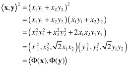
defining a 3-D feature space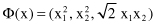 . Similar analysis may be performed for other kernel function. For example, through the similar process verify that for the “full” quadratic kernel (
2
the feature space is 6-D.
Figure 4.25.
An example of a mapping Φ to a feature space in which the data become linearly separable. (a) One-dimensional input space; (b) two-dimensional feature space.
In practical use of SVM, only the kernel function
k
(and not transformation function Φ) is specified. The selection of an appropriate kernel function is important, since the kernel function defines the feature space in which the training set examples will be classified. As long as the kernel function is legitimate, an SVM will operate correctly even if the designer does not know exactly what features of the training data are being used in the kernel-induced feature space. The definition of a legitimate kernel function is given by Mercer’s theorem: The function must be continuous and positive-definite.
Modified and enhanced SVM constructs an optimal separating hyperplane in the higher dimensional space. In this case, the optimization problem becomes
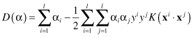
where
K(x,y)
is the kernel function performing the nonlinear mapping into the feature space, and the constraints are unchanged. Using kernel function we will perform minimization of dual Lagrangian in the feature space, and determine all margin parameter, without representing points in this new space. Consequently, everything that has been derived concerning the linear case is also applicable for a nonlinear case by using a suitable kernel
K
instead of the dot product.
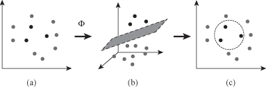
The approach with kernel functions gives a modular SVM methodology. One module is always the same: Linear Learning Module. It will find margin for linear separation of samples. If the problem of classification is more complex, requiring nonlinear separation, then we include a new preparatory module. This module is based on kernel function, and it transforms input space into higher, feature space where the same Linear Learning Module may be applied, and the final solution is nonlinear classification model. Illustrative example is given in Figure
4.26
. This combination of different kernel functions with standard SVM learning algorithm for linear separation gives the flexibility to the SVM methodology for efficient application in nonlinear cases.
Figure 4.26.
SVM performs nonlinear classification by kernel-based transformations. (a) 2-D input space; (b) 3-D feature space; (c) 2-D input space.
The idea of using a hyperplane to separate the feature vectors into two groups works well when there are only two target categories, but how does SVM handle the case where the target variable has more than two categories? Several approaches have been suggested, but two are the most popular: (a) “one against many” where each category is split out and all of the other categories are merged; and (b) “one against one” where
k
(
k
− 1)/2 models are constructed and
k
is the number of categories.
A preparation process for SVM applications is enormously important for the final results, and it includes preprocessing of raw data and setting model parameters. SVM requires that each data sample is represented as a vector of real numbers. If there are categorical attributes, we first have to convert them into numeric data. Multi-attribute coding is recommended in this case. For example, a three-category attribute such as red, green, and blue can be represented with three separate attributes and corresponding codes such as (0,0,1), (0,1,0), and (1,0,0). This approach is appropriate only if the number of values in an attribute is not too large. Second, scaling values of all numerical attributes before applying SVM is very important in successful application of the technology. The main advantage is to avoid attributes with greater numeric ranges to dominate those in smaller ranges. Normalization for each attribute may be applied to the range [−1; +1] or [0; 1].
Selection of parameters for SVM is very important and the quality of results depends on these parameters. Two most important parameters are cost C and parameter γ for Gaussian kernel. It is not known beforehand which C and σ are the best for one problem; consequently, some kind of parameter search must be done. The goal is to identify good (C; σ) so that the classifier can accurately predict unknown data (i.e., testing data). Note that it may not be required to achieve high-training accuracy. Small cost C is appropriate for close to linear separable samples. If we select small C for nonlinear classification problem, it will cause under-fitted learning. Large C for nonlinear problems is appropriate, but not too much because the classification margin will become very thin resulting in over-fitted learning. Similar analysis is for Gaussian kernel σ parameter. Small σ will cause close to linear kernel with no significant transformation in future space and less flexible solutions. Large σ generates extremely complex nonlinear classification solution.
The experience in many real-world SVM applications suggests that, in general, RBF model is a reasonable first choice. The RBF kernel nonlinearly maps samples into a higher dimensional space, so, unlike the linear kernel, it can handle the case when the relation between classes is highly nonlinear. The linear kernel should be treated a special case of RBF. The second reason for RBF selection is the number of hyper-parameters that influences the complexity of model selection. For example, polynomial kernels have more parameters than the RBF kernel and the tuning proves is much more complex and time-consuming. However, there are some situations where the RBF kernel is not suitable, and one may just use the linear kernel with extremely good results. The question is when to use the linear kernel as a first choice. If the number of features is large, one may not need to map data to a higher dimensional space. Experiments showed that the nonlinear mapping does not improve the SVM performance. Using the linear kernel is good enough, and C is the only tuning parameter. Many microarray data in bioinformatics and collection of electronic documents for classification are examples of this data set type. As the number of features is smaller, and the number of samples increases, SVM successfully maps data to higher dimensional spaces using nonlinear kernels.
One of the methods for finding optimal parameter values for an SVM is a grid search. The algorithm tries values of each parameter across the specified search range using geometric steps. Grid searches are computationally expensive because the model must be evaluated at many points within the grid for each parameter. For example, if a grid search is used with 10 search intervals and an RBF kernel function is used with two parameters (C and σ), then the model must be evaluated at 10*10 = 100 grid points, that is, 100 iterations in a parameter-selection process.
At the end we should highlight main strengths of the SVM methodology. First, a training process is relatively easy with a small number of parameters and the final model is never presented with local optima, unlike some other techniques. Also, SVM methodology scales relatively well to high-dimensional data and it represents a trade-off between a classifier’s complexity and accuracy. Nontraditional data structures like strings and trees can be used as input samples to SVM, and the technique is not only applicable to classification problems, it is also accommodated for prediction. Weaknesses of SVMs include computational inefficiency and the need to experimentally choose a “good” kernel function.
The SVM methodology is becoming increasingly popular in the data-mining community. Software tools that include SVM are becoming more professional, user-friendly, and applicable to many real-world problems where data sets are extremely large. It has been shown that SVM outperforms other techniques such as logistic regression or artificial neural networks on a wide variety of real-world problems. Some of the most successful applications of the SVM have been in image processing, in particular handwritten digit recognition and face recognition. Other interesting application areas for SVMs are in text mining and categorization of large collection of documents, and in the analysis of genome sequences in bioinformatics. Furthermore, the SVM has been successfully used in a study of text and data for marketing applications. As kernel methods and maximum margin methods including SVM are further improved and taken up by the data-mining community, they are becoming an essential tool in any data miner’s tool kit.