Authors: Mehmed Kantardzic
Data Mining (28 page)

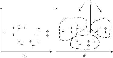
Figure 4.12.
Graphical interpretation of clustering. (a) Training data set; (b) description of clusters.
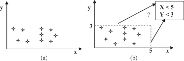
Summarization
is also a typical descriptive task, where the inductive-learning process is without a teacher. It involves methods for finding a
compact description
for a set (or subset) of data. If a description is formalized, as given in Figure
4.13
b, that information may simplify and therefore improve the decision-making process in a given domain.
Figure 4.13.
Graphical interpretation of summarization. (a) Training data set; (b) formalized description.
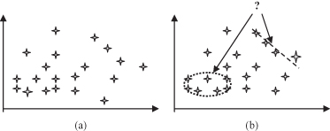
Dependency modeling
is a learning task that discovers local models based on a training data set. The task consists of finding a model that describes significant dependency between features or between values in a data set covering not the entire data set, but only some specific subsets. An illustrative example is given in Figure
4.14
b, where the ellipsoidal relation is found for one subset and a linear relation for the other subset of the training data. These types of modeling are especially useful in large data sets that describe very complex systems. Discovering general models based on the entire data set is, in many cases, almost impossible, because of the computational complexity of the problem at hand.
Figure 4.14.
Graphical interpretation of dependency-modeling task. (a) Training data set; (b) discovered local dependencies.
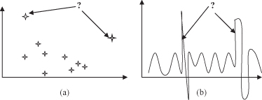
Change and deviation detection
is a learning task, and we have been introduced already to some of its techniques in Chapter 2. These are the algorithms that detect outliers. In general, this task focuses on discovering the most significant changes in a large data set. Graphical illustrations of the task are given in Figure
4.15
. In Figure
4.15
a the task is to discover outliers in a given data set with discrete values of features. The task in Figure
4.15
b is detection of time-dependent deviations for the variable in a continuous form.
Figure 4.15.
Graphical interpretation of change and detection of deviation (a) Outliers; (b) changes in time.
The list of inductive-learning tasks is not exhausted with these six classes that are common specifications for data-mining problems. With wider and more intensive applications of the data-mining technology, new specific tasks are being developed, together with the corresponding techniques for inductive learning.
Whatever the learning task and whatever the available data-mining techniques are, we have to accept that the foundation for successful data-mining processes is data-preprocessing and data-reduction methods. They transform raw and usually messy data into valuable data sets for mining, using methodologies explained in Chapters 2 and 3. As a review, we will enumerate some of these techniques just to show how many alternatives the data-mining designer has in the beginning phases of the process: scaling and normalization, encoding, outliers detection and removal, feature selection and composition, data cleansing and scrubbing, data smoothing, missing-data elimination, and cases reduction by sampling.
When the data are preprocessed and when we know what kind of learning task is defined for our application, a list of data-mining methodologies and corresponding computer-based tools are available. Depending on the characteristics of the problem at hand and the available data set, we have to make a decision about the application of one or more of the data-mining and knowledge-discovery techniques, which can be classified as follows:
1.
Statistical Methods.
The typical techniques are Bayesian inference, logistic regression, analysis of variance (ANOVA), and log-linear models.
2.
Cluster Analysis.
The common techniques of which are divisible algorithms, agglomerative algorithms, partitional clustering, and incremental clustering.
3.
Decision Trees and Decision Rules.
The set of methods of inductive learning developed mainly in artificial intelligence. Typical techniques include the Concept Learning System (CLS) method, the ID3 algorithm, the C4.5 algorithm, and the corresponding pruning algorithms.
4
Association Rules.
They represent a set of relatively new methodologies that include algorithms such as market basket analysis, a priori algorithm, and WWW path-traversal patterns.
5.
Artificial Neural Networks.
The common examples of which are multilayer perceptrons with backpropagation learning and Kohonen networks.
6.
Genetic Algorithms.
They are very useful as a methodology for solving hard-optimization problems, and they are often a part of a data-mining algorithm.
7.
Fuzzy Inference Systems.
These are based on the theory of fuzzy sets and fuzzy logic. Fuzzy modeling and fuzzy decision making are steps very often included in a data-mining process.
8.
N-dimensional Visualization Methods.
These are usually skipped in the literature as a standard data-mining methodology, although useful information may be discovered using these techniques and tools. Typical data-mining visualization techniques are geometric, icon-based, pixel-oriented, and hierarchical.
This list of data-mining and knowledge-discovery techniques is not exhaustive, and the order does not suggest any priority in the application of these methods. Iterations and interactivity are basic characteristics of these data-mining techniques. Also, with more experience in data-mining applications, the reader will understand the importance of not relying on a single methodology. Parallel application of several techniques that cover the same inductive-learning task is a standard approach in this phase of data mining. In that case, for each iteration in a data-mining process, the results of the different techniques must additionally be evaluated and compared.
4.5 SVMs
The foundations of SVMs have been developed by Vladimir Vapnik and are gaining popularity due to many attractive features, and promising empirical performance. The formulation embodies the SRM principle. SVMs were developed to solve the classification problem, but recently they have been extended to the domain of regression problems (for prediction of continuous variables). SVMs can be applied to regression problems by the introduction of an alternative loss function that is modified to include a distance measure. The term SVM is referring to both classification and regression methods, and the terms Support Vector Classification (SVC) and Support Vector Regression (SVR) may be used for more precise specification.
An SVM is a supervised learning algorithm creating learning functions from a set of labeled training data. It has a sound theoretical foundation and requires relatively small number of samples for training; experiments showed that it is insensitive to the number of samples’ dimensions. Initially, the algorithm addresses the general problem of learning to discriminate between members of two classes represented as n-dimensional vectors. The function can be a classification function (the output is binary) or the function can be a general regression function.
SVM’s classification function is based on the concept of decision planes that define decision boundaries between classes of samples. A simple example is shown in Figure
4.16
a where the samples belong either to class gray or black. The separating line defines a boundary on the right side of which all samples are gray, and to the left of which all samples are black. Any new unclassified sample falling to the right will be classified as gray (or classified as black should it fall to the left of the separating line).
Figure 4.16.
Linear separation in a 2-D space. (a) Decision plane in 2-D space is a line. (b) How to select optimal separating line?
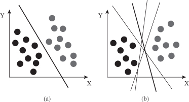
The classification problem can be restricted to consideration of the two-class problem without loss of generality. Before considering n-dimensional analysis, let us look at a simple 2-D example. Assume that we wish to perform a classification, and our data has a categorical target variable with two categories. Also assume that there are two input attributes with continuous values. If we plot the data points using the value of one attribute on the x-axis and the other on the y-axis, we might end up with an image such as shown in the Figure
4.16
b. In this problem the goal is to separate the two classes by a function that is induced from available examples. The goal is to produce a classifier that will work well on unseen examples, that is, it generalizes well. Consider the data in Figure
4.16
b. Here there are many possible linear classifiers that can separate the two classes of samples. Are all decision boundaries equally good? How do we prove that the selected one is the best?
The main idea is: The decision boundary should be as far away as possible from the data points of both classes. There is only one that maximizes the margin (maximizes the distance between it and the nearest data point of each class). Intuitively, the margin is defined as the amount of space, or separation between the two classes as defined by the hyperplane. Geometrically, the margin corresponds to the shortest distance between the closest data points to a point on the hyperplane. SLT suggests that the choice of the maximum margin hyperplane will lead to maximal generalization when predicting the classification of previously unseen examples.