Data Mining (31 page)
Authors: Mehmed Kantardzic

The SVM learning algorithm is defined so that, in a typical case, the number of SVs is small compared with the total number of training examples. This property allows the SVM to classify new examples efficiently, since the majority of the training examples can be safely ignored. SVMs effectively remove the uninformative patterns from the data set by assigning them α
i
weights of 0. So, if internal points that are not SVs are changed, no effect will be made on the decision boundary. The hyperplane is represented sparsely as a linear combination of “SV” points. The SVM automatically identifies a subset of these informative points and uses them to represent the solution.
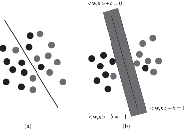
In real-world applications, SVMs must deal with (a) handling the cases where subsets cannot be completely separated, (b) separating the points with nonlinear surfaces, and (c) handling classifications with more than two categories. Illustrative examples are given in Figure
4.22
. What are solutions in these cases? We will start with the problem of data that are not linearly separable. The points such as shown on the Figure
4.23
a could be separated only by a nonlinear region. Is it possible to define a linear margin where some points may be on opposite sides of hyperplanes?
Figure 4.22.
Issues for an SVM in real-world applications. (a) Subset cannot be completely separated; (b) nonlinear separation; (c) three categories.

Figure 4.23.
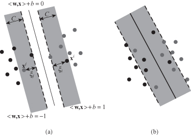
Soft margin SVM. (a) Soft separating hyperplane; (b) error points with their distances.

Obviously, there is no hyperplane that separates all of the samples in one class from all of the samples in the other class. In this case there would be no combination of w and b that could ever satisfy the set of constraints. This situation is depicted in Figure
4.23
b, where it becomes apparent that we need to
soften
the constraint that these data lay on the correct side of the +1 and −1 hyperplanes. We need to allow some, but not too many data points to violate these constraints by a preferably small amount. This alternative approach turns out to be very useful not only for datasets that are not linearly separable, but also, and perhaps more importantly, in allowing improvements in generalization. We modify the optimization problem including cost of violation factor for samples that violate constraints:

under new constraints:

where
C
is a parameter representing the cost of violating the constraints, and
ξ
i
are distances of samples that violate constraints. To allow some flexibility in separating the categories, SVM models introduce a cost parameter,
C
, that controls the trade-off between allowing training errors and forcing rigid margins. It creates a
soft margin
(as the one in Figure
4.24
) that permits some misclassifications. If
C
is too small, then insufficient stress will be placed on fitting the training data. Increasing the value of
C
increases the cost of misclassifying points and forces the creation of a more accurate model that may not generalize well.
Figure 4.24.
Trade-off between allowing training errors and forcing rigid margins. (a) Parameters
C
and X for a soft margin; (b) soft classifier with a fat margin (
C
> 0).

This SVM model is a very similar case to the previous optimization problem for the linear separable data, except that there is an upper bound
C
on all α
i
parameters. The value of
C
trades between how large of a margin we would prefer, as opposed to how many of the training set examples violate this margin (and by how much). The process of optimization is going through the same steps: Lagrangian, optimization of α
i
parameters, and determining
w
and
b
values for classification hyperplane. The dual stay the same, but with additional constraints on α parameters: 0 ≤ α
i
≤ C.
Most classification tasks require more complex models in order to make an optimal separation, that is, correctly classify new test samples on the basis of the trained SVM. The reason is that the given data set requires nonlinear separation of classes. One solution to the inseparability problem is to map the data into a higher dimensional space and define a separating hyperplane there. This higher dimensional space is called the
feature space
, as opposed to the
input space
occupied by the training samples. With an appropriately chosen feature space of sufficient dimensionality, any consistent training set can be made linearly separable. However, translating the training set into a higher dimensional space incurs both computational and learning costs. Representing the feature vectors corresponding to the training set can be extremely expensive in terms of memory and time. Computation in the feature space can be costly because it is high-dimensional. Also, in general, there is the question of which function is appropriate for transformation. Do we have to select from infinite number of potential functions?
There is one characteristic of the SVM optimization process that helps in determining the steps in the methodology. The SVM decision function for classifying points with respect to the hyperplane only involves dot products between points. Furthermore, the algorithm that finds a separating hyperplane in the feature space can be stated entirely in terms of vectors in the input space and dot products in the feature space. We are transforming training samples from one space into the other. But we are making computation only with scalar products of points in this new space. This product is computationally inexpensive because only a small subset of points is SVs involved in product computation. Thus, an SVM can locate a separating hyperplane in the feature space and classify points in that space without ever representing the space explicitly, simply by defining a function, called a
kernel function
. Kernel function
K
always plays the role of the dot product in the feature space:

This approach avoids the computational burden of explicitly representing all transformed source data and high-dimensional feature vectors. The two most widely used kernel functions are Polynomial Kernel

and Gaussian Kernel
