Authors: Mehmed Kantardzic
Data Mining (36 page)

The lift chart is also a big help in evaluating the usefulness of a model. It shows how responses are changed in percentiles of testing samples population, by applying the data mining model. For example, in Figure
4.32
a, instead of a 10% response rate when a random 10% of the population is treated, the response rate of the top selected 10% of the population is over 35%. The lift is 3.5 in this case.
Another important component of interpretation is to assess the financial benefits of the model. Again, a discovered model may be interesting and relatively accurate, but acting on it may cost more than the revenue or savings it generates. The Return on Investment (ROI) chart, given in Figure
4.32
b, is a good example of how attaching values to a response and costs to a program can provide additional guidance to decision making. Here, ROI is defined as ratio of profit to cost. Note that beyond the eighth decile (80%), or 80% of testing population, the ROI of the scored model becomes negative. It is at a maximum for this example at the second decile (20% of population).
We can explain the interpretation and practical use of lift and ROI charts on a simple example of a company who wants to advertise their products. Suppose they have a large database of addresses for sending advertising materials. The question is: Will they send these materials to everyone in the database? What are the alternatives? How do they obtain the maximum profit from this advertising campaign? If the company has additional data about “potential” costumers in their database, they may build the predictive (classification) model about the behavior of customers and their responses to the advertisement. In estimation of the classification model, lift chart is telling the company what the potential improvements in advertising results are. What are benefits if they use the model and based on the model select only the most promising (responsive) subset of database instead of sending ads to everyone? If the results of the campaign are presented in Figure
4.32
a the interpretation may be the following. If the company is sending the advertising materials to the top 10% of customers selected by the model, the expected response will be 3.5 times greater than sending the same ads to randomly selected 10% of customers. On the other hand, sending ads involves some cost and receiving response and buying the product results in additional profit for the company. If the expenses and profits are included in the model, ROI chart shows the level of profit obtained with the predictive model. From Figure
4.32
b it is obvious that the profit will be negative if ads are sent to all customers in the database. If it is sent only to 10% of the top customers selected by the model, ROI will be about 70%. This simple example may be translated to large number of different data-mining applications.
While lift and ROI charts are popular in the business community for evaluation of data-mining models, the scientific community “likes” the Receiver Operating Characteristic (ROC) curve better. What is the basic idea behind an ROC curve construction? Consider a classification problem where all samples have to be labeled with one of two possible classes. A typical example is a diagnostic process in medicine, where it is necessary to classify the patient as being with or without disease. For these types of problems, two different yet related error rates are of interest. The False Acceptance Rate (FAR) is the ratio of the number of test cases that are incorrectly “accepted” by a given model to the total number of cases. For example, in medical diagnostics, these are the cases in which the patient is wrongly predicted as having a disease. On the other hand, the False Reject Rate (FRR) is the ratio of the number of test cases that are incorrectly “rejected” by a given model to the total number of cases. In the previous medical example, these are the cases of test patients who are wrongly classified as healthy.
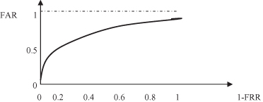
For the most of the available data-mining methodologies, a classification model can be tuned by setting an appropriate threshold value to operate at a desired value of FAR. If we try to decrease the FAR parameter of the model, however, it would increase the FRR and vice versa. To analyze both characteristics at the same time, a new parameter was developed, the ROC curve. It is a plot of FAR versus 1 − FRR for different threshold values in the model. This curve permits one to assess the performance of the model at various operating points (thresholds in a decision process using the available model) and the performance of the model as a whole (using as a parameter the area below the ROC curve). The ROC curve is especially useful for a comparison of the performances of two models obtained by using different data-mining methodologies. The typical shape of an ROC curve is given in Figure
4.33
where the axes are
sensitivity
(FAR) and
1-specificity
(1 − FRR).
Figure 4.33.
The ROC curve shows the trade-off between sensitivity and 1-specificity values.
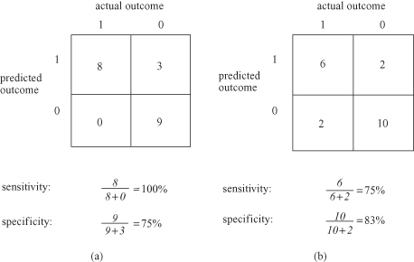
How does one construct an ROC curve in practical data-mining applications? Of course, many data-mining tools have a module for automatic computation and visual representation of an ROC curve. What if this tool is not available? At the beginning we are assuming that we have a table with actual classes and predicted classes for all training samples. Usually, predicted values as an output from the model are not computed as 0 or 1 (for two class problem) but as real values on interval [0, 1]. When we select a threshold value, we may assume that all predicted values above the threshold are 1, and all values below the threshold are 0. Based on this approximation we may compare actual class with predicted class by constructing a confusion matrix, and compute sensitivity and specificity of the model for the given threshold value. In general, we can compute sensitivity and specificity for large numbers of different threshold values. Every pair of values (sensitivity, 1-specificity) represents one discrete point on a final ROC curve. Examples are given in Figure
4.34
. Typically, for graphical presentation, we are systematically selecting threshold values. For example, starting from 0 and increasing by 0.05 until 1, we have 21 different threshold values. That will generate enough points to reconstruct an ROC curve.
Figure 4.34.
Computing points on an ROC curve. (a) Threshold = 0.5; (b) threshold = 0.8.
When we are comparing two classification algorithms we may compare the measures as accuracy or F measure, and conclude that one model is giving better results than the other. Also, we may compare lift charts, ROI charts, or ROC curves, and if one curve is above the other we may conclude that a corresponding model is more appropriate. But in both cases we may not conclude that there are significant differences between models, or more important, that one model shows better performances than the other with statistical significance. There are some simple tests that could verify these differences. The first one is McNemar’s test. After testing models of both classifiers, we are creating a specific contingency table based on classification results on testing data for both models. Components of the contingency table are explained in Table
4.5
.
TABLE 4.5.
Contingency Table for McNemar’s Test
| e 00 : Number of samples misclassified by both classifiers | e 01 : Number of samples misclassified by classifier 1, but not classifier 2 |
| e 10 : Number of samples misclassified by classifier 2, but not classifier 1 | e 11 : Number of samples correctly classified by both classifier s |
After computing the components of the contingency table, we may apply the χ
2
statistic with one degree of freedom for the following expression:
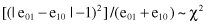
McNemar’s test rejects the hypothesis that the two algorithms have the same error at the significance level α, if previous value is greater than χ
2
α, 1
. For example, for α = 0.05, χ
2
0.05, 1
= 3.84.
The other test is applied if we compare two classification models that are tested with the K-fold cross-validation process. The test starts with the results of K-fold cross-validation obtained from K training/validation set pairs. We compare the error percentages in two classification algorithms based on errors in K validation sets that are recorded for two models as: and
and , i = 1, … , K.
The difference in error rates on fold i is . Then, we can compute: