Data Mining (102 page)
Authors: Mehmed Kantardzic


An episode is a partially ordered set of events. When the order among the events of an episode is total, it is called a
serial
episode, and when there is no order at all, the episode is called a
parallel
episode. For example, (
A
→
B
→
C
) is a three-node serial episode. The arrows in our notation serve to emphasize the total order. In contrast, parallel episodes are somewhat similar to itemsets, and so, we can denote a three-node parallel episode with event types
A
,
B
, and
C
, as (
ABC
).
An episode is said to
occur
in an event sequence if there exist events in the sequence occurring with exactly the same order as that prescribed in the episode. For instance, in the example the events (
A,
2), (
B,
3) and (
C,
8) constitute an occurrence of the serial episode (
A
→
B
→
C
) while the events (
A,
7), (
B,
3), and (
C,
8) do not, because for this serial episode to occur,
A
must occur before
B
and
C
. Both these sets of events, however, are valid occurrences of the parallel episode (
ABC
), since there are no restrictions with regard to the order in which the events must occur for parallel episodes. Let
α
and
β
be two episodes.
β
is said to be a
sub-episode
of
α
if all the event types in
β
appear in
α
as well, and if the partial order among the event types of
β
is the same as that for the corresponding event types in
α
. For example, (
A
→
C
) is a two-node sub-episode of the serial episode (
A
→
B
→
C
) while (
B
→
A
) is not. In case of parallel episodes, this order constraint is not required.
The sequential pattern-mining framework may extend the frequent itemsets idea described in the chapter on association rules with temporal order. The database
D of itemsets
is considered no longer just some unordered collection of transactions. Now, each transaction in
D
carries a time stamp as well as a customer ID. Each transaction, as earlier, is simply a collection of items. The transactions associated with a single customer can be regarded as a sequence of itemsets ordered by time, and
D
would have one such transaction sequence corresponding to each customer. Consider an example database with five customers whose corresponding transaction sequences are as follows:
| Customer ID | Transaction Sequence |
| 1 | ({ A,B }{ A,C,D }{ B,E }) |
| 2 | ({ D,G } { A,B,E,H }) |
| 3 | ({ A }{ B,D }{ A,B,E,F }{ G,H }) |
| 4 | ({ A }{ F }) |
| 5 | ({ A,D } { B,E,G,H } { F }) |
Each customer’s transaction sequence is enclosed in angular braces, while the items bought in a single transaction are enclosed in round braces. For example, customer 3 made four visits to the supermarket. In his/her first visit he/she bought only item
A
, in the second visit items
B
and
D
, and so on.
The temporal patterns of interest are sequences of itemsets. A sequence
S
of itemsets is denoted by {
s
1
s
2
· · ·
s
n
}, where
s
j
is an itemset. Since
S
has
n
itemsets, it is called an
n
-sequence. A sequence
A
= {
a
1
a
2
· · ·
a
n
} is said to be
contained in
another sequence
B
= {
b
1
b
2
· · ·
b
m
} if there exist integers
i
1
<
i
2
<
· · ·
<
i
n
such that
a
1
⊆
b
i
1
, a
2
⊆
b
i
2
, . . ., a
n
⊆
b
in
. That is, an
n
-sequence
A
is contained in a sequence
B
if there exists an
n
-length subsequence in
b
, in which each itemset contains the corresponding itemsets of
a
. For example, the sequence {
(A)(BC)
} is contained in {
(AB) (F) (BCE) (DE)
} but not in {
(BC) (AB) (C) (DEF)
}. Further, a sequence is said to be
maximal
in a set of sequences, if it is not contained in any other sequence. In the set of example customer-transaction sequences listed above, all are maximal (with respect to the given set of sequences) except the sequence of customer 4, which is contained in transaction sequences of customers 3 and 5.
The Apriori algorithm described earlier can be used to find frequent sequences, except that there is a small difference in the definition of support. Earlier, the support of an itemset was defined as the fraction of
all
transactions that contained the itemset. Now, the
support
for any arbitrary sequence
A
is the fraction of customer transaction sequences in the database
D
, which contains
A
. For our example database, the sequence {
(D)(GH)
} has a support of 0.4, since it is contained in two out of the five transaction sequences (namely, that of customer 3 and customer 5). The user specifies a minimum support threshold. Any sequence of itemsets with support greater than or equal to the threshold value is called a
large
sequence. If a sequence
A
is large and maximal, then it is regarded as a
sequential pattern
. The process of frequent episode discovery is an Apriori-style iterative algorithm that starts with discovering frequent one-element sequences. These are then combined to form candidate two-element sequences, and then by counting their frequencies, two-element frequent sequences are obtained. This process is continued till frequent sequences of all lengths are found. The task of a sequence mining is to systematically discover all sequential patterns in database
D
.
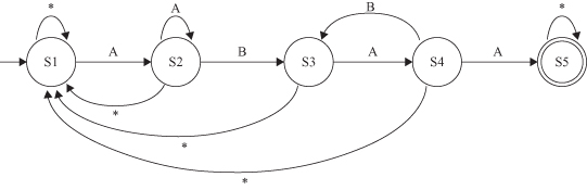
Counting frequencies of parallel itemsets is straightforward and described in traditional algorithms for frequent itemsets detection. Counting serial itemsets, on the other hand, requires more computational resources. For example, unlike for parallel itemsets, we need finite-state automata to recognize serial episodes. More specifically, an appropriate
l
-state automaton can be used to recognize occurrences of an
l
-node serial sequence. For example, for the sequence
(A
→
B → A → A)
, there would be a five-state automaton (FSA) given in Figure
12.23
. It transits from its first state on seeing an event of type
A
and then waits for an event of type
B
to transit to its next state, and so on. We need such automata for each episode whose frequency is being counted.
Figure 12.23.
FSA for the sequence A → B → A → A. *, any other symbol.
While we described the framework using an example of mining a database of customer transaction sequences for temporal buying patterns, this concept of sequential patterns is quite general and can be used in many other situations as well. Indeed, the problem of motif discovery in a database of protein sequences can also be easily addressed in this framework. Another example is Web-navigation mining. Here the database contains a sequence of Web sites that a user navigates through in each browsing session. Sequential pattern mining can be used to discover sequences of Web sites that are frequently visited. Temporal associations are particularly appropriate as candidates for causal rules’ analysis in temporally related medical data, such as in the histories of patients’ medical visits. Patients are associated with both static properties, such as gender, and temporal properties, such as age, symptoms, or current medical treatments. Adapting this method to deal with temporal information leads to some different approaches. A possible extension is a new meaning for a typical association rule X ≥ Y. It states now that if X occurs, then Y will occur within time T. Stating a rule in this new form allows for controlling the impact of the occurrence of one event to the other event occurrence, within a specific time interval. In case of the sequential patterns framework some generalizations are proposed to incorporate minimum and maximum time-gap constraints between successive elements of a sequential pattern.
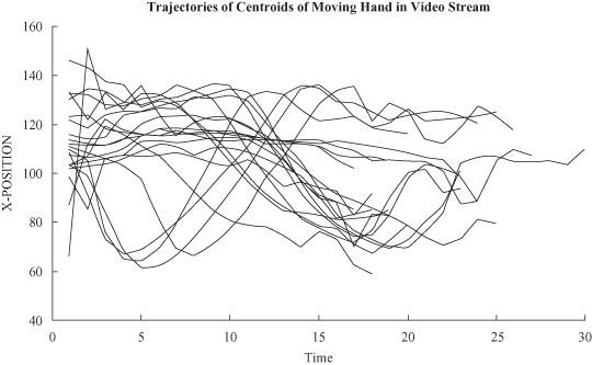
Mining continuous data streams is a new research topic related to temporal data mining that has recently received significant attention. The term “data stream” pertains to data arriving over time, in a nearly continuous fashion. It is often a fast-changing stream with a huge number of multidimensional data (Fig.
12.24
). Data are collected close to their source, such as sensor data, so they are usually with a low level of abstraction. In streaming data-mining applications, the data are often available for mining only once, as it flows by. That causes several challenging problems, including how to aggregate the data, how to obtain scalability of traditional analyses in massive, heterogeneous, nonstationary data environment, and how to incorporate incremental learning into a data-mining process. Linear, single-scan algorithms are still rare in commercial data-mining tools, but also still challenged in a research community. Many applications, such as network monitoring, telecommunication applications, stock market analysis, bio-surveillance systems, and distribute sensors depend critically on the efficient processing and analysis of data streams. For example, a frequent itemset-mining algorithm over data stream is developed. It is based on an incremental algorithm to maintain the FP stream, which is a tree data structure to represent the frequent itemsets and their dynamics in time.
Figure 12.24.
Multidimensional streams.