Data Mining (100 page)
Authors: Mehmed Kantardzic

Once the break points are defined along with the corresponding coding symbols for each interval, the sequence is discretized as follows:
1.
Obtain the PAA averages of the time series.
2.
All PAA averages in the given interval ( ,
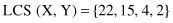
, ) are coded with a specific symbol for this interval. For example, if α = 3, all PAA averages less than the smallest break point (−0.43) are mapped to “
a.
” All PAA coefficients less than the second break point but greater than first breakpoint (−0.43, 0.43) are mapped to “
b
,” and all average values larger than the second break point (0.43) are mapped to “
c.
” This process is illustrated in Figure
12.18
.
Figure 12.18.
Transformation of PAA to SAX.
It is assumed that the symbols “
a
,” “
b
,” and “
c
” are approximately equiprobable symbols in the representation of a time series. The original sequence is then represented as a concatenation of these symbols, which is known as a “word.” For example, the mapping from PAA (
C′
) to a word
C″
is represented as
C″
= (
bcccccbaaaaabbccccbb
). The main advantage of the SAX method is that 100 different discrete numerical values in an initial discrete time series C is first reduced to 20 different (average) values using PAA, and then they are transformed into only three different categorical values using SAX.

The proposed approach is intuitive and simple, yet a powerful methodology in a simplified representation of a large number of different values in time series. The method is fast to compute and supports different distance measures. Therefore, it is applicable as a data-reduction step for different data-mining techniques.
Transformation-Based Representations
The main idea behind transformation-based techniques is to map the original data into a point of a more manageable domain. One of the widely used methods is the
Discrete Fourier Transformation
(DFT). It transforms a sequence in the time domain to a point in the frequency domain. This is done by selecting the top-K frequencies and representing each sequence as a point in the K-dimensional space. One important property that is worth noting is that Fourier coefficients do not change under the shift operation. One problem with DFT is that it misses the important feature of time localization. To avoid this problem
Piecewise Fourier Transform
was proposed, but the size of the pieces introduced new problems. Large pieces reduce the power of multi-resolution, while modeling of low frequencies with small pieces does not always give expected representations. The
Discrete Wavelet Transformation
(DWT) has been introduced to overcome the difficulties in DFT. The DWT transformation technique, analogously to fast Fourier transformation, turns a discrete vector of function values with the length N into a vector of N wavelet coefficients. Wavelet transformation is a linear operation and it is usually implemented as a recursion. The advantage of using DWT is its ability for multi-resolution representation of signals. It has the time-frequency localization property. Therefore, signals represented by wavelet transformations bear more information than that of DFT.
In some applications we need to retrieve objects from a database of certain shapes. Trends can often be reflected by specifying shapes of interest such as steep peaks, or upward and downward changes. For example, in a stock-market database we may want to retrieve stocks whose closing price contains a
head-and-shoulders
pattern, and we should be able to represent and recognize this shape. Pattern discovery can be driven by a template-based mining language in which the analyst specifies the shape that should be looked for.
Shape Definition Language
(SDL) was proposed to translate the initial sequence with real-valued elements occurring in historical data into a sequence of symbols from a given alphabet. SDL is capable of describing a variety of queries about the shapes found in the database. It allows the user to create his or her own language with complex patterns in terms of primitives. More interestingly, it performs well on approximate matching, where the user cares only about the overall shape of the sequence but not about specific details. The first step in the representation process is defining the alphabet of symbols and then translating the initial sequence to a sequence of symbols. The translation is done by considering sample-to-sample transitions, and then assigning a symbol of the described alphabet to each transition.
A significantly different approach is to convert a sequence into discrete representation by using
clustering
. A sliding window of width
w
is used to generate subsequences from the original sequence. These subsequences are then clustered, considering the pattern similarity between subsequences, using a suitable clustering method, for example, the
k
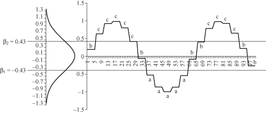
-nearest neighbor method. A different symbol is then assigned to each cluster. The discrete version of the time series is obtained by using cluster identities corresponding to the subsequence. For example, the original time sequence is defined with integer values given in time: (1, 2, 3, 2, 3, 4, 3, 4, 3, 4, 5, 4, 5) as represented in Figure
12.19
a. The Window width is defined by three consecutive values, and samples of primitives are collected through the time series. After simplified clustering, the final set of three “frequent” primitive shapes, representing cluster centroids, is given in Figure
12.19
b. Assigning symbolic representation for these shapes, a
1
, a
2
, and a
3
, the final symbolic representation of the series will be (a
3
, a
2
, a
1
, a
1
, a
3
, a
2
).
Figure 12.19.
Clustering approach in primitive shapes discovery. (a) Time series; (b) primitive shapes after clustering.
12.2.2 Similarity Measures between Sequences
The individual elements of the sequences may be vectors of real numbers (e.g., in applications involving speech or audio signals) or they may be symbolic data (e.g., in applications involving gene sequences). After representing each sequence in a suitable form, it is necessary to define a similarity measure between sequences, in order to determine if they match. Given two sequences T
1
and T
2
, we need to define an appropriate similarity function
Sim
, which calculates the closeness of the two sequences, denoted by
Sim
(T
1
, T
2
). Usually, the similarity measure is expressed in terms of inverse distance measure, and for various types of sequences and applications, we have numerous distance measures. An important issue in measuring similarity between two sequences is the ability to deal with outlying points, noise in the data, amplitude differences causing
scaling problems
, and the existence of gaps and other time-distortion problems. The most straightforward distance measure for time series is the Euclidean distance and its variants, based on the common Lp-norms. It is used in time-domain continuous representations by viewing each sub-sequence with
n
discrete values as a point in R
n
. Besides being relatively straightforward and intuitive, Euclidean distance and its variants have several other advantages. The complexity of evaluating these measures is linear; they are easy to implement, indexable with any access method, and, in addition, are parameter-free. Furthermore, the Euclidean distance is surprisingly competitive with other more complex approaches, especially if the size of the training set/database is relatively large. However, since the mapping between the points of two time series is fixed, these distance measures are very sensitive to noise and misalignments in time, and are unable to handle local-time shifting, that is, similar segments that are out of phase.
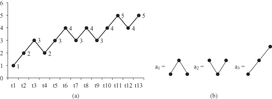
When a sequence is represented as a sequence of discrete symbols of an alphabet, the similarity between two sequences is achieved most of the time by comparing each element of one sequence with the corresponding one in the other sequence. The best known such distance is the longest common subsequence (LCS) similarity, utilizing the search for the LCS in both sequences we are comparing, and normalized with the length of the longer sequence. For example, if two sequences X and Y are given as X = {10, 5, 6, 9, 22, 15, 4, 2} and Y = {6, 5, 10, 22, 15, 4, 2, 6, 8}, then the LCS is