Data Mining (98 page)
Authors: Mehmed Kantardzic

By specifying a “minimum support” value, subgraphs Gs, whose support values are above threshold, are mined as candidates or components of candidates for maximum frequent subgraphs. The main difference in an a priori implementation is that we need to define the join process of two subgraphs a little differently. Two graphs of size k can be joined if they have a structure of size (k − 1) in common. The
size of this structure
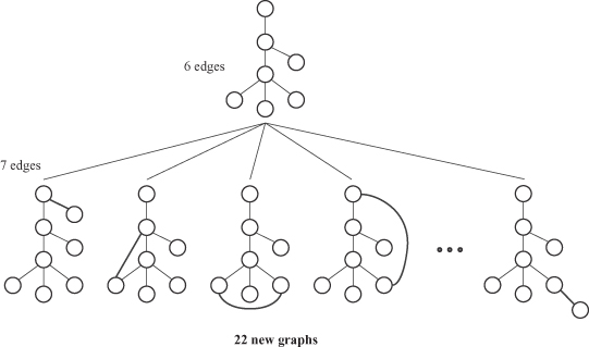
could be defined in terms of either nodes or edges. The algorithm starts by finding all frequent single- and double-link subgraphs. Then, in each iteration, it generates candidate subgraphs by expanding the subgraphs found in the previous iteration by one edge. The algorithm checks how many times the candidate subgraph with the extension occurs within an entire graph or set of graphs. The candidates whose frequency is below a user-defined level are pruned. The algorithm returns all subgraphs occurring more frequently than the given threshold. A naïve approach of a subgraph extension from kk − 1 size to size k is computationally very expensive as illustrated in Figure
12.12
. Therefore, the candidate generation of a frequently induced subgraph is done with some constraints. Two frequent graphs are joined only when the following conditions are satisfied to generate a candidate of frequent graph of size k + 1. Let X
k
and Y
k
be adjacency matrices of two frequent graphs G(X
k
) and G(Y
k
) of size k. If both G(X
k
) and G(Y
k
) have equal elements of the matrices except for the elements of the
k
th row and the
k
th column, then they may be joined to generate Z
k
+
1
as an adjacency matrix for a candidate graph of size k + 1.
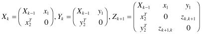
Figure 12.12.
Free extensions in graphs.
In this matrix representations, X
k−1
is the common adjacency matrix representing the graph whose size is kk − 1, while x
i
and y
i
(i = 1, 2) are (kk − 1) × 1 column vectors. These column vectors represent the differences between two graphs prepared for the join operation.
The process suffers from computational intractability when the graph size becomes too large. One problem is subgraph
isomorphism,
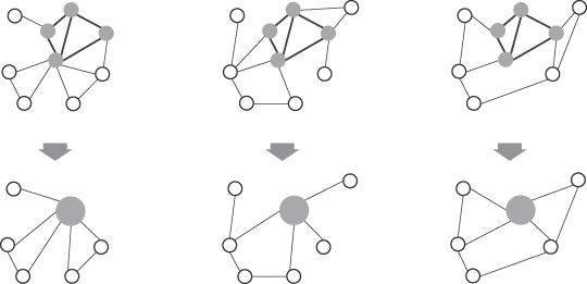
with NP complexity, as a core step in graph matching. Also, all frequent patterns may not be equally relevant in the case of graphs. In particular, patterns that are highly connected (which means dense subgraphs) are much more relevant. This additional analysis requires more computations. One possible application of discovering frequent subgraphs is a summarized representation of larger, complex graphs. After extracting common subgraphs, it is possible to simplify large graphs by condensing these subgraphs into new nodes. An illustrative example is given in Figure
12.13
,
where a subgraph of four nodes is replaced in the set of graphs with a single node. The resulting graphs represent summarized representation of the initial graph set.
Figure 12.13.
Graph summarization through graph compression.
In recent years, significant attention has focused on studying the structural properties of networks such as the WWW, online social networks, communication networks, citation networks, and biological networks. Across these large networks, an important characteristic is that they can be characterized by the nature of the underlying graphs and subgraphs, and clustering is an often used technique for miming these large networks. The problem of graph clustering arises in two different contexts: a single large graph or large set of smaller graphs. In the first case, we wish to determine dense node clusters in a
single large graph
minimizing the intercluster similarity for a fixed number of clusters. This problem arises in the context of a number of applications such as graph partitioning and the minimum-cut problem. The determination of dense regions in the graph is a critical problem from the perspective of a number of different applications in social networks and Web-page summarization. Top-down clustering algorithms are closely related to the concept of
centrality analysis
in graphs where central nodes are typically key members in a network that is well connected to other members of the community. Centrality analysis can also be used in order to determine the central points in information flows. Thus, it is clear that the same kind of structural-analysis algorithm can lead to different kinds of insights in graphs. For example, if the criterion for separating a graph into subgraphs is a maximum measure of link betweenness, then the graph in Figure
12.14
a may be transformed into six subgraphs as presented in Figure
12.14
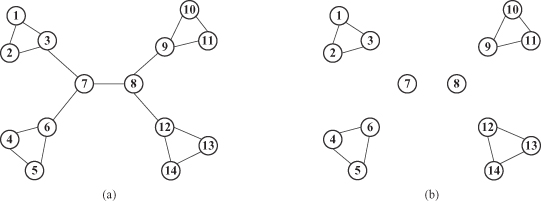
b. In this case the maximum betweenness of 49 was for the link (7, 8), and elimination of this link defines two clusters on the highest level of hierarchy. The next value of betweenness, 33, was found for links (3,7), (8, 9), (6, 7), and (8, 12). After elimination of these links on the second level of hierarchy, the graph is decomposed into six dense subgraphs of clustered nodes.
Figure 12.14.
Graph clustering using betweenness measure. (a) Initial graph; (b) subgraphs after elimination of links with maximum betweenness.
The second case of cluster analysis assumes multiple graphs, each of which may possibly be of modest size. These large number of graphs need to be clustered based on their underlying structural behavior. The problem is challenging because of the need to match the structures of the underlying graphs, and these structures are used for clustering purposes. The main idea is that we wish to cluster graphs as objects, and the distance between graphs is defined based on a structural similarity function such as the edit distance. This clustering approach makes it an ideal technique for applications in areas such as scientific-data exploration, information retrieval, computational biology, Web-log analysis, forensics analysis, and blog analysis.
Link analysis is an important field that has received a lot of attention recently when advances in information technology enabled mining of extremely large networks. The basic data structure is still a graph, only the emphasis in analysis is on links and their characteristics: labeled or unlabeled, directed or undirected. There is an inherent ambiguity with respect to the term “link” that occurs in many circumstances, but especially in discussions with people whose background and research interests are in the database community. In the database community, especially the subcommunity that uses the well-known entity-relationship (ER) model, a “link” is a connection between two records in two different tables. This usage of the term “link” in the database community differs from that in the intelligence community and in the artificial intelligence (AI) research community. Their interpretation of a “link” typically refers to some real world connection between two entities. Probably the most famous example of exploiting link structure in the graph is the use of links to improve information retrieval results. Both, the well-known PageRank measure and hubs, and authority scores are based on the link structure of the Web. Link analysis techniques are used in law enforcement, intelligence analysis, fraud detection, and related domains. It is sometimes described using the metaphor of “connecting the dots” because link diagrams show the connections between people, places, events, and things, and represent invaluable tools in these domains.
12.2 TEMPORAL DATA MINING
Time is one of the essential natures of data. Many real-life data describe the property or status of some object at a particular time instance. Today time-series data are being generated at an unprecedented speed from almost every application domain, for example, daily fluctuations of stock market, traces of dynamic processes and scientific experiments, medical and biological experimental observations, various readings obtained from sensor networks, Web logs, computer-network traffic, and position updates of moving objects in location-based services. Time series or, more generally, temporal sequences, appear naturally in a variety of different domains, from engineering to scientific research, finance, and medicine. In engineering matters, they usually arise with either sensor-based monitoring, such as telecommunication control, or log-based systems monitoring. In scientific research they appear, for example, in spatial missions or in the genetics domain. In health care, temporal sequences have been a reality for decades, with data originated by complex data-acquisition systems like electrocardiograms (ECGs), or even simple ones like measuring a patient’s temperature or treatment effectiveness. For example, a supermarket transaction database records the items purchased by customers at some time points. In this database, every transaction has a time stamp in which the transaction is conducted. In a telecommunication database, every signal is also associated with a time. The price of a stock at the stock market database is not constant, but changes with time as well.
Temporal databases capture attributes whose values change with time. Temporal data mining is concerned with data mining of these large data sets. Samples related with the temporal information present in this type of database need to be treated differently from static samples. The accommodation of time into mining techniques provides a window into the temporal arrangement of events and, thus, an ability to suggest cause and effect that are overlooked when the temporal component is ignored or treated as a simple numeric attribute. Moreover, temporal data mining has the ability to mine the behavioral aspects of objects as opposed to simply mining rules that describe their states at a point in time. Temporal data mining is an important extension as it has the capability of mining activities rather than just states and, thus, inferring relationships of contextual and temporal proximity, some of which may also indicate a cause–effect association.
Temporal data mining
is concerned with data mining of large sequential data sets. By sequential data, we mean data that are ordered with respect to some index. For example, a time series constitutes a popular class of sequential data where records are indexed by time. Other examples of sequential data could be text, gene sequences, protein sequences, Web logs, and lists of moves in a chess game. Here, although there is no notion of time as such, the ordering among the records is very important and is central to the data description/modeling. Sequential data include: