Data Mining (99 page)
Authors: Mehmed Kantardzic

1.
Temporal Sequences.
They represent ordered series of nominal symbols from a particular alphabet (e.g., a huge number of relatively short sequences in Web-log files or a relatively small number of extremely long gene expression sequences). This category includes ordered but not time stamped collections of samples. The sequence relationships include before, after, meet, and overlap.
2.
Time Series.
It represents a time-stamped series of continuous, real-valued elements (e.g., a relatively small number of long sequences of multiple sensor data or monitoring recordings from digital medical devices). Typically, most of the existing work on time series assumes that time is discrete. Formally, time-series data are defined as a sequence of pairs T = ([p
1
, t
1
], [p
2
, t
2
], … , [p
n
, t
n
]), where t
1
< t
2
< … < t
n
. Each p
i
is a data point in a d-dimensional data space, and each t
i
is the time stamp at which p
i
occurs. If the sampling rate of a time series is constant, one can omit the time stamps and consider the series as a sequence of d-dimensional data points. Such a sequence is called the raw representation of the time series.
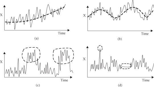
Traditional analyses of temporal data require a statistical approach because of noise in raw data, missing values, or incorrect recordings. They include (1) long-term trend estimation, (2) cyclic variations, for example, business cycles, (3) seasonal patterns, and (4) irregular movements representing outliers. Examples are given in Figure
12.15
. The discovery of relations in temporal data requires more emphasis in a data-mining process on the following three steps: (1) the representation and modeling of the data sequence in a suitable form; (2) the definition of similarity measures between sequences; and (3) the application of variety of new models and representations to the actual mining problems.
Figure 12.15.
Traditional statistical analyses of time series. (a) Trend; (b) cycle; (c) seasonal; (d) outliers.
12.2.1 Temporal Data Representation
The representation of temporal data is especially important when dealing with large volumes of data since direct manipulation of continuous, high-dimensional data in an efficient way is extremely difficult. There are a few ways this problem can be addressed.
Original Data or with Minimal Preprocessing
Use data as they are without or with minimal preprocessing. We preserve the characteristics of each data point when a model is built. The main disadvantage of this process is that it is extremely inefficient to build data-mining models with millions of records of temporal data, all of them with different values.
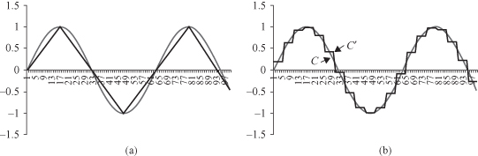
Windowing and Piecewise Approximations
There is well-known psychological evidence that the human eye segments smooth curves into piecewise straight lines. Based on this theory, there are a number of algorithms for segmenting a curve that represents a time series. Figure
12.16
shows a simple example where it replaces the original nonlinear function with several piecewise linear functions. As shown in the figure, the initial real-valued elements (time series) are partitioned into several segments. Finding the required number of segments that best represent the original sequence is not trivial. An easy approach is to predefine the number of segments. A more realistic approach may be to define them when a change point is detected in the original sequence. Another technique based on the same idea segments a sequence by iteratively merging two similar segments. Segments to be merged are selected based on the squared-error minimization criteria. Even though these methods have the advantage of ability to reduce the impact of noise in the original sequence, when it comes to real-world applications (e.g., sequence matching) differences in amplitudes (scaling) and time-axis distortions are not addressed easily.
Figure 12.16.
Simplified representation of temporal data. (a) Piecewise linear approximation; (b) piecewise aggregate approximation.
To overcome these drawbacks,
Piecewise Aggregate Approximation
(PAA) technique was introduced. It approximates the original data by segmenting the sequences into same-length sections and recording the mean value of these sections. A time-series
C
of length
n
is represented as
C
= {c
1
, c
2
, … , c
n
}. The task is to represent
C
as
C′
in a
w
-dimensional space (w <
n
) by mean values of c
i
s in w equal-sized segments. The
i
th element of
C′
is calculated as a mean of all values in the segment:
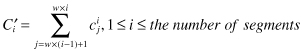
For example, if the original sequence is C = {−2, −4, −3, −1, 0, 1, 2, 1, 1, 0}, where n = |C| = 10, and we decide to represent
C
in two sections of the same length, then


Usually, PAA is visualized as a linear combination of box bases functions as illustrated in Figure
12.16
b, where a continuous function is replaced with 10 discrete averages for each interval.
A modified PAA algorithm, which is called
Symbolic Aggregate Approximation
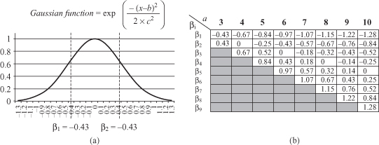
(SAX), is proposed with the assumption that the original normalized time series,
C
, has a Gaussian distribution of PAA values. SAX defines “break points” in the Gaussian curve that will produce equal-sized areas below the curve. Formally, break points are a sorted list of numbers such that the areas under the Gaussian curve from
 to
to are equal to 1/α, and they are constant. α is a parameter of the methodology representing the number of intervals. These break points can be determined in a statistical table. For example, Figure
12.17
gives the break points for α values from 3 to 10.
Figure 12.17.
SAX look-up table. (a) Break points in the Gaussian curve (
b
= 0,
c
2
= 0.2) when α = 3; (b) SAX look-up table.