Data Mining (47 page)
Authors: Mehmed Kantardzic

In general, the hypothesis H
0
is rejected at the level of significance α if

where T(α) is the threshold value from the χ
2
distribution table usually given in textbooks on statistics. For our example, selecting α = 0.05 we obtain the threshold

A simple comparison shows that
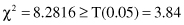
and therefore, we can conclude that hypothesis H
0
is rejected; the attributes analyzed in the survey have a high level of dependency. In other words, the attitude about abortion shows differences between the male and the female populations.
The same procedure may be generalized and applied to contingency tables where the categorical attributes have more than two values. The next example shows how the previously explained procedure can be applied without modifications to the contingency table 3 × 3. The values given in Table
5.7a
are compared with the estimated values given in Table
5.7b
, and the corresponding test is calculated as χ
2
= 3.229. Note that in this case parameter

TABLE 5.7.
Contingency Tables for Categorical Attributes with Three Values
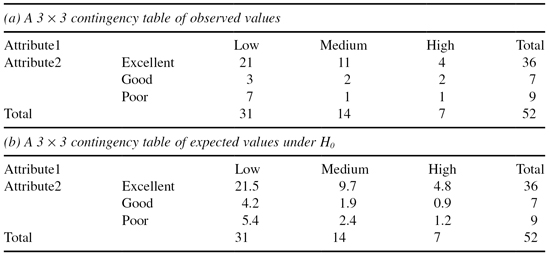
We have to be very careful about drawing additional conclusions and further analyzing the given data set. It is quite obvious that the sample size is not large. The number of observations in many cells of the table is small. This is a serious problem and additional statistical analysis is necessary to check if the sample is a good representation of the total population or not. We do not cover this analysis here because in most real-world data-mining problems the data set is enough large to eliminate the possibility of occurrence of these deficiencies.
That was one level of generalization for an analysis of contingency tables with categorical data. The other direction of generalization is inclusion into analysis of more than two categorical attributes. The methods for three- and high-dimensional contingency table analysis are described in many books on advanced statistics; they explain the procedure of discovered dependencies between several attributes that are analyzed simultaneously.
5.8 LDA
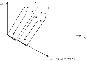
LDA is concerned with classification problems where the dependent variable is categorical (nominal or ordinal) and the independent variables are metric. The objective of LDA is to construct a discriminant function that yields different scores when computed with data from different output classes. A linear discriminant function has the following form:
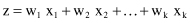
where x
1
, x
2
, … , x
k
are independent variables. The quantity z is called the discriminant score, and w
1
, w
2
, … ,w
k
are called weights. A geometric interpretation of the discriminant score is shown in Figure
5.5
. As the figure shows, the discriminant score for a data sample represents its projection onto a line defined by the set of weight parameters.
Figure 5.5.
Geometric interpretation of the discriminant score.
The construction of a discriminant function z involves finding a set of weight values w
i
that maximizes the ratio of the
between-class
to the
within-class
variance of the discriminant score for a preclassified set of samples. Once constructed, the discriminant function z is used to predict the class of a new nonclassified sample. Cutting scores serve as the criteria against which each individual discriminant score is judged. The choice of cutting scores depends upon a distribution of samples in classes. Letting z
a
and z
b
be the mean discriminant scores of preclassified samples from class A and B, respectively, the optimal choice for the cutting score z
cut-ab
is given as
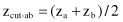
when the two classes of samples are of equal size and are distributed with uniform variance. A new sample will be classified to one or another class depending on its score z > z
cut-ab
or z < z
cut-ab
. A weighted average of mean discriminant scores is used as an optimal cutting score when the set of samples for each of the classes are not of equal size:
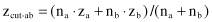
The quantities n
a
and n
b
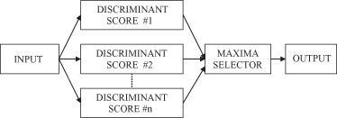
represent the number of samples in each class. Although a single discriminant function z with several discriminant cuts can separate samples into several classes,
multiple discriminant analysis
is used for more complex problems. The term multiple discriminant analysis is used in situations when separate discriminant functions are constructed for each class. The classification rule in such situations takes the following form: Decide in favor of the class whose discriminant score is the highest. This is illustrated in Figure
5.6
.
Figure 5.6.
Classification process in multiple-discriminant analysis.