Authors: Mehmed Kantardzic
Data Mining (45 page)


where n is the number of input dimensions, m is the number of samples, Y
j
is a vector with dimensions c × 1, and c is the number of outputs. This multivariate model can be fitted in exactly the same way as a linear model using least-square estimation. One way to do this fitting would be to fit a linear model to each of the c dimensions of the output, one at a time. The corresponding residuals for each dimension will be (y
j
− y’
j
) where y
j
is the exact value for a given dimension and y’
j
is the estimated value.
The analog of the residual sum of squares for the univariate linear model is the matrix of the residual sums of squares for the multivariate linear model. This matrix R is defined as
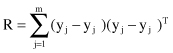
The matrix R has the residual sum of squares for each of the c dimensions stored on its leading diagonal. The off-diagonal elements are the residual sums of cross-products for pairs of dimensions. If we wish to compare two nested linear models to determine whether certain β’s are equal to 0, then we can construct an extra sum of squares matrix and apply a method similar to ANOVA—MANOVA. While we had an F-statistic in the ANOVA methodology, MANOVA is based on matrix R with four commonly used test statistics: Roy’s greatest root, the Lawley-Hotteling trace, the Pillai trace, and Wilks’ lambda. Computational details of these tests are not explained in the book, but most textbooks on statistics will explain these; also, most standard statistical packages that support MANOVA support all four statistical tests and explain which one to use under what circumstances.
Classical multivariate analysis also includes the method of principal component analysis, where the set of vector samples is transformed into a new set with a reduced number of dimensions. This method has been explained in Chapter 3 when we were talking about data reduction and data transformation as preprocessing phases for data mining.
5.6 LOGISTIC REGRESSION
Linear regression is used to model continuous-value functions. Generalized regression models represent the theoretical foundation on that the linear regression approach can be applied to model categorical response variables. A common type of a generalized linear model is
logistic regression
. Logistic regression models the probability of some event occurring as a linear function of a set of predictor variables.
Rather than predicting the value of the dependent variable, the logistic regression method tries to estimate the probability that the dependent variable will have a given value. For example, in place of predicting whether a customer has a good or bad credit rating, the logistic regression approach tries to estimate the probability of a good credit rating. The actual state of the dependent variable is determined by looking at the estimated probability. If the estimated probability is greater than 0.50 then the prediction is closer to
YES
(a good credit rating), otherwise the output is closer to
NO
(a bad credit rating is more probable). Therefore, in logistic regression, the probability p is called the success probability.
We use logistic regression only when the output variable of the model is defined as a categorical binary. On the other hand, there is no special reason why any of the inputs should not also be quantitative, and, therefore, logistic regression supports a more general input data set. Suppose that output Y has two possible categorical values coded as 0 and 1. Based on the available data we can compute the probabilities for both values for the given input sample: P(y
j
= 0) = 1 − p
j
and P(y
j
= 1) = p
j
. The model with which we will fit these probabilities is accommodated linear regression:

This equation is known as the
linear logistic model
. The function log (p
j
/[1−p
j
]) is often written as
logit(p).
The main reason for using the logit form of output is to prevent the predicting probabilities from becoming values out of the required range [0, 1]. Suppose that the estimated model, based on a training data set and using the linear regression procedure, is given with a linear equation

and also suppose that the new sample for classification has input values {x
1
, x
2
, x
3
} = {1, 0, 1}. Using the linear logistic model, it is possible to estimate the probability of the output value 1, (p[Y = 1]) for this sample. First, calculate the corresponding logit(p):

and then the probability of the output value 1 for the given inputs:
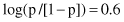
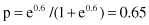
Based on the final value for probability p, we may conclude that output value Y = 1 is more probable than the other categorical value Y = 0. Even this simple example shows that logistic regression is a very simple yet powerful classification tool in data-mining applications. With one set of data (training set) it is possible to establish the logistic regression model and with other sets of data (testing set) we may analyze the quality of the model in predicting categorical values. The results of logistic regression may be compared with other data-mining methodologies for classification tasks such as decision rules, neural networks, and Bayesian classifier.
5.7 LOG-LINEAR MODELS
Log-linear modeling is a way of analyzing the relationship between categorical (or quantitative) variables. The log-linear model approximates discrete, multidimensional probability distributions. It is a type of a generalized linear model where the output Yi is assumed to have a Poisson distribution, with expected value μ
j
. The natural logarithm of μ
j
is assumed to be the linear function of inputs

Since all the variables of interest are categorical variables, we use a table to represent them, a frequency table that represents the global distribution of data. The aim in log-linear modeling is to identify associations between categorical variables. Association corresponds to the interaction terms in the model, so our problem becomes a problem of finding out which of all β’s are 0 in the model. A similar problem can be stated in ANOVA. If there is an interaction between the variables in a log-linear mode, it implies that the variables involved in the interaction are not independent but related, and the corresponding β is not equal to 0. There is no need for one of the categorical variables to be considered as an output in this analysis. If the output is specified, then instead of the log-linear models, we can use logistic regression for analysis. Therefore, we will next explain log-linear analysis when a data set is defined without output variables. All given variables are categorical, and we want to analyze the possible associations between them. That is the task for
correspondence analysis
.