Data Mining (43 page)
Authors: Mehmed Kantardzic

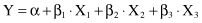
where α, β
1
, β
2
, and β
3
are coefficients that are found by using the method of least squares. For a linear regression model with more than two input variables, it is useful to analyze the process of determining β parameters through a matrix calculation:

where β = {β
0
, β
1
, … , β
n
}, β
0
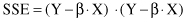
= α, and X and Y are input and output matrices for a given training data set. The residual sum of the squares of errors SSE will also have the matrix representation
and after optimization

the final β vector satisfies the matrix equation
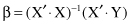
where β is the vector of estimated coefficients in a linear regression. Matrices X and Y have the same dimensions as the training data set. Therefore, an optimal solution for β vector is relatively easy to find in problems with several hundreds of training samples. For real-world data-mining problems, the number of samples may increase to several millions. In these situations, because of the extreme dimensions of matrices and the exponentially increased complexity of the algorithm, it is necessary to find modifications and/or approximations in the algorithm, or to use totally different regression methods.
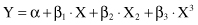
There is a large class of regression problems, initially nonlinear, that can be converted into the form of the general linear model. For example, a polynomial relationship such as

can be converted to the linear form by setting new variables X
4
= X
1
· X
3
and X
5
= X
2
· X
3
. Also, polynomial regression can be modeled by adding polynomial terms to the basic linear model. For example, a cubic polynomial curve has a form
By applying transformation to the predictor variables (X
1
= X, X
2
= X
2
, and X
3
= X
3
), it is possible to linearize the model and transform it into a multiple-regression problem, which can be solved by the method of least squares. It should be noted that the term linear in the general linear model applies to the dependent variable being a linear function of the unknown parameters. Thus, a general linear model might also include some higher order terms of independent variables, for example, terms such as X
1
2
, e
βX
, X
1
·X
2
, 1/X, or X
2
3
. The basis is, however, to select the proper transformation of input variables or their combinations. Some useful transformations for linearization of the regression model are given in Table
5.3
.
TABLE 5.3.
Some Useful Transformations to Linearize Regression
| Function | Proper Transformation | Form of Simple |
| | | Linear Regression |
| Exponential: | ||
| Y = α e βx | Y* = ln Y | Regress Y* against x |
| Power: | ||
| Y = α x β | Y* = logY; x* = log x | Regress Y* against x* |
| Reciprocal: | ||
| Y = α + β(1/x) | x* = 1/x | Regress Y against x* |
| Hyperbolic: | ||
| Y = x/(α + βx) | Y* = 1/Y; x* = 1/x | Regress Y* against x* |
The major effort, on the part of a user, in applying multiple-regression techniques lies in identifying the
relevant
independent variables from the initial set and in selecting the regression model using only relevant variables. Two general approaches are common for this task:
1.
Sequential Search Approach.
It is consists primarily of building a regression model with an initial set of variables and then selectively adding or deleting variables until some overall criterion is satisfied or optimized.
2.
Combinatorial Approach.
It is, in essence, a brute-force approach, where the search is performed across all possible combinations of independent variables to determine the best regression model.
Irrespective of whether the sequential or combinatorial approach is used, the maximum benefit to model building occurs from a proper understanding of the application domain.
Additional postprocessing steps may estimate the quality of the linear regression model. Correlation analysis attempts to measure the strength of a relationship between two variables (in our case this relationship is expressed through the linear regression equation). One parameter, which shows this strength of linear association between two variables by means of a single number, is called a
correlation coefficient r
. Its computation requires some intermediate results in a regression analysis.
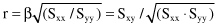
where
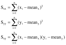
The value of r is between −1 and 1. Negative values for r correspond to regression lines with negative slopes and a positive r shows a positive slope. We must be very careful in interpreting the r value. For example, values of r equal to 0.3 and 0.6 only mean that we have two positive correlations, the second somewhat stronger than the first. It is wrong to conclude that r = 0.6 indicates a linear relationship twice as strong as that indicated by the value r = 0.3.