Data Mining (106 page)
Authors: Mehmed Kantardzic

12.5 CORRELATION DOES NOT IMPLY CAUSALITY
An associational concept is any relationship that can be defined in terms of a frequency-based joint distribution of observed variables, while a causal concept is any relationship that cannot be defined from the distribution alone. Even simple examples show that the associational criterion is neither necessary nor sufficient for causality confirmation. For example, data mining might determine that males with income between $50,000 and $65,000 who subscribe to certain magazines are likely purchasers of a product you want to sell. While you can take advantage of this pattern, say by aiming your marketing at people who fit the pattern, you should not assume that any of these factors (income, type of magazine)
cause
them to buy your product. The predictive relationships found via data mining are not necessarily
causes
of an action or behavior.
The research questions that motivate many studies in the health, social, and behavioral sciences are not statistical but causal in nature. For example, what is the efficacy of a given drug in a given population, or what fraction of past crimes could have been avoided by a given policy? The central target of such studies is to determine cause–effect relationships among variables of interests, for example, treatments–diseases or policies–crime, as precondition–outcome relationships. In order to express causal assumptions mathematically, certain extensions are required in the standard mathematical language of statistics, and these extensions are not generally emphasized in the mainstream literature and education.
The aim of standard statistical analysis, typified by regression and other estimation techniques, is to infer parameters of a distribution from samples drawn from that distribution. With the help of such parameters, one can infer associations among variables, or estimate the likelihood of past and future events. These tasks are managed well by standard statistical analysis so long as experimental conditions remain the same. Causal analysis goes one step further; its aim is to infer aspects of the data-generation process. Associations characterize static conditions, while causal analysis deals with changing conditions. There is nothing in the joint distribution of symptoms and diseases to tell us that curing the former would or would not cure the latter.
Drawing analogy to visual perception, the information contained in a probability function is analogous to a geometrical description of a three-dimensional object; it is sufficient for predicting how that object will be viewed from any angle outside the object, but it is insufficient for predicting how the object will be deformed if manipulated and squeezed by external forces. The additional information needed for making predictions such as the object’s resilience or elasticity is analogous to the information that causal assumptions provide. These considerations imply that the slogan “correlation does not imply causation” can be translated into a useful principle: One cannot substantiate causal claims from associations alone, even at the population level. Behind every causal conclusion there must lie some causal assumptions that are not testable in observational studies.
Any mathematical approach to causal analysis must acquire a new notation for expressing causal assumptions and causal claims. To illustrate, the syntax of probability calculus does not permit us to express the simple fact that “symptoms do not cause diseases,” let alone draw mathematical conclusions from such facts. All we can say is that two events are dependent—meaning that if we find one, we can expect to encounter the other, but we cannot distinguish statistical dependence, quantified by the conditional probability
P
(
disease/symptom
) from causal dependence, for which we have no expression in standard probability calculus. Symbolic representation for the relation “symptoms cause disease” is distinct from the symbolic representation of “symptoms are associated with disease.”
The need to adopt a new notation, foreign to the province of probability theory, has been traumatic to most persons trained in statistics partly because the adaptation of a new language is difficult in general, and partly because statisticians—this author included—have been accustomed to assuming that all phenomena, processes, thoughts, and modes of inference can be captured in the powerful language of probability theory. Causality formalization requires new mathematical machinery for cause–effect analysis and a formal foundation for counterfactual analysis including concepts such as “path diagrams,” “controlled distributions,” causal structures, and causal models.
12.5.1 Bayesian Networks
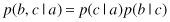
One of the powerful aspects of graphical models is that a specific graph can make probabilistic statements for a broad class of distributions. In order to motivate the use of directed graphs to describe probability distributions, consider first an arbitrary joint distribution p(a, b, c) over three variables a, b, and c. By application of the product rule of probability, we can write the joint distribution in the form

We now represent the right-hand side of the equation in terms of a simple graphical model as follows. First, we introduce a node for each of the random variables a, b, and c and associate each node with the corresponding conditional distribution on the right-hand side of the equation. Then, for each conditional distribution we add directed links, (arrows) to the graph from the nodes corresponding to the variables on which the distribution is conditioned. Thus, for the factor p(c|a, b), there will be links from nodes a and b to node c, whereas for the factor p(a) there will be no incoming links, as presented in Figure
12.33
a. If there is a link going from a node a to a node b, then we say that node
a
is the
parent
of node b, and we say that node b is the
child
of node
a
.
Figure 12.33.
A directed graphical model representing the joint probability distribution over a set of variables. (a) Fully connected; (b) partially connected.
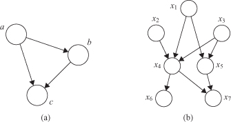
For given K variables, we can again represent a joint probability distribution as a directed graph having K nodes, one for each conditional distribution, with each node having incoming links from all lower numbered nodes. We say that this graph is
fully connected
because there is a link between every pair of nodes. Consider now the graph shown in Figure
12.33
b, which is not a fully connected graph because, for instance, there is no link from x
1
to x
2
or from x
3
to x
7
. We may transform this graph to the corresponding representation of the joint probability distribution written in terms of the product of a set of conditional distributions, one for each node in the graph. The joint distribution of all seven variables is given by

Any joint distribution can be represented by a corresponding graphical model. It is the
absence
of links in the graph that conveys interesting information about the properties of the class of distributions that the graph represents. We can interpret such models as expressing the processes by which the observed data arose, and in many situations we may draw conclusions about new samples from a given probability distribution. The directed graphs that we are considering are subject to an important restriction, that is, that there must be no
directed cycles
. In other words, there are no closed paths within the graph such that we can move from node to node along links following the direction of the arrows and end up back at the starting node. Such graphs are also called
Directed Acyclic Graphs
(
DAGs
).
An important concept for probability distributions over multiple variables is that of
conditional independence.
Consider three variables a, b, and c, and suppose that the conditional distribution of a, given b and c, is such that it does not depend on the value of b, so that
We say that
a
is conditionally independent of
b
given
c
. This can be extended in a slightly different way if we consider the joint distribution of
a
and
b
conditioned on
c
, which we can write in the form

The joint distribution of
a
and
b
, conditioned on
c
, may be factorized into the product of the marginal distribution of
a
and the marginal distribution of
b
(again both conditioned on
c
). This says that the variables
a
and
b
are statistically independent, given
c
. This independence may be presented in a graphical form in Figure
12.34
a. The other typical joint distributions may be graphically interpreted. The distribution for Figure
12.34
b represents the case