Data Mining (67 page)
Authors: Mehmed Kantardzic

The simplest neighborhood function, which refers to a neighborhood set of nodes around the BMU node
i
, is a monotonically decreasing Gaussian function:
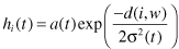
where
α
(
t
) is a learning rate (0 < α(t) < 1), and the width of the kernel
σ
(
t
) is a monotonically decreasing function of time as well, and
t
is the current time step (iteration of the loop). While the process will adapt all weight vectors within the current neighborhood region, including those of the winning neuron, those outside this neighborhood are left unchanged. The initial radius is set high, some values near the width or height of the map. As a result, at the early stage of training when the neighborhood is broad and covers almost all the neurons, the self-organization takes place at the global scale. As the iterations continue, the base goes toward the center, so there are fewer neighbors as time progresses. At the end of training, the neighborhood shrinks to 0 and only BMU neuron updates its weights. The network will generalize through the process to organize similar vectors (which it has not previously seen) spatially close at the SOM outputs.
Apart from reducing the neighborhood, it has also been found that quicker convergence of the SOM algorithm is obtained if the adaptation rate of nodes in the network is reduced over time. Initially the adaptation rate should be high to produce coarse clustering of nodes. Once this coarse representation has been produced, however, the adaptation rate is reduced so that smaller changes to the weight vectors are made at each node and regions of the map become fine-tuned to the input-training vectors. Therefore, every node within the BMU’s neighborhood including the BMU has its weight vector adjusted through the learning process. The previous equation for weight factors correction
h
i
(
t
) may include an exponential decrease of “winner’s influence” introducing
α
(
t
) also as a monotonically decreasing function.
The number of output neurons in an SOM (i.e., map size) is important to detect the deviation of the data. If the map size is too small, it might not explain some important differences that should be detected between input samples. Conversely, if the map size is too big, the differences are too small. In practical applications, if there is no additional heuristics, the number of output neurons in an SOM can be selected using iterations with different SOM architectures.
The main advantages of SOM technology are as follows: presented results are very easy to understand and interpret; technology is very simple for implementation; and most important, it works well in many practical problems. Of course, there are also some disadvantages. SOMs are computationally expensive; they are very sensitive to measure of similarity; and finally, they are not applicable for real-world data sets with missing values. There are several possible improvements in implementations of SOMs. To reduce the number of iterations in a learning process, good initialization of weight factors is essential.
Principal components of input data
can make computation of the SOM orders of magnitude faster. Also, practical experience shows that hexagonal grids give output results with a better quality. Finally, selection of distance measure is important as in any clustering algorithm. Euclidean distance is almost standard, but that does not mean that it is always the best. For an improved quality (isotropy) of the display, it is advisable to select the grid of the SOM units as
hexagonal
.
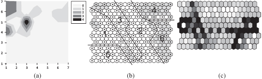
The SOMs have been used in large spectrum of applications such as automatic speech recognition, clinical data analysis, monitoring of the condition of industrial plants and processes, classification from satellite images, analysis of genetic information, analysis of electrical signals from the brain, and retrieval from large document collections. Illustrative examples are given in Figure
7.18
.
Figure 7.18.
SOM applications. (a) Drugs binding to human cytochrome; (b) interest rate classification; (c) analysis of book-buying behavior.
7.8 REVIEW QUESTIONS AND PROBLEMS
1.
Explain the fundamental differences between the design of an ANN and “classical” information-processing systems.
2.
Why is fault-tolerance property one of the most important characteristics and capabilities of ANNs?
3.
What are the basic components of the neuron’s model?
4.
Why are continuous functions such as log-sigmoid or hyperbolic tangent considered common activation functions in real-world applications of ANNs?
5.
Discuss the differences between feedforward and recurrent neural networks.
6.
Given a two-input neuron with the following parameters: bias b = 1.2, weight factors W = [w1, w2] = [3, 2], and input vector X = [−5, 6]
T
; calculate the neuron’s output for the following activation functions:
(a)
a symmetrical hard limit
(b)
a log-sigmoid
(c)
a hyperbolic tangent
7.
Consider a two-input neuron with the following weight factors W and input vector X:
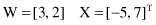
We would like to have an output of 0.5.
(a)
Is there a transfer function from Table 9.1 that will do the job if the bias is zero?
(b)
Is there a bias that will do the job if the linear-transfer function is used?
(c)
What is the bias that will do the job with a log-sigmoid–activation function?
8.
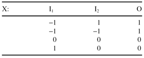
Consider a classification problem defined with the set of 3-D samples X, where two dimensions are inputs and the third one is the output.
(a)
Draw a graph of the data points X labeled according to their classes. Is the problem of classification solvable with a single-neuron perceptron? Explain the answer.
(b)
Draw a diagram of the perceptron you would use to solve the problem. Define the initial values for all network parameters.
(c)
Apply single iteration of the delta-learning algorithm. What is the final vector of weight factors?
9. The one-neuron network is trained to classify input–output samples:
| 1 | 0 | 1 |
| 1 | 1 | −1 |
| 0 | 1 | 1 |
Show that this problem cannot be solved unless the network uses a bias.
10.
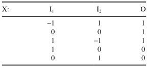
Consider the classification problem based on the set of samples X:
(a)
Draw a graph of the data points labeled according to their classification. Is the problem solvable with one artificial neuron? If yes, graph the decision boundaries.
(b)
Design a single-neuron perceptron to solve this problem. Determine the final weight factors as a weight vector orthogonal to the decision boundary.
(c)
Test your solution with all four samples.
(d)
Using your network classify the following samples: (−2, 0), (1, 1), (0, 1), and (−1, −2).
(e)
Which of the samples in (d) will always be classified the same way, and for which samples classification may vary depending on the solution?
11.
Implement the program that performs the computation (and learning) of a single-layer perceptron.
12.
For the given competitive network:
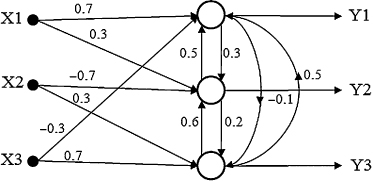
(a)
find the output vector [Y1, Y2, Y3] if the input sample is [X1, X2, X3] = [1, −1, −1];
(b)
what are the new weight factors in the network?
13.
Search the Web to find the basic characteristics of publicly available or commercial software tools that are based on ANNs. Document the results of your search. Which of them are for learning with a teacher, and which are support learning without a teacher?
14.
For a neural network, which one of these structural assumptions is the one that most affects the trade-off between underfitting (i.e., a high-bias model) and overfitting (i.e., a high-variance model):