Data Mining (71 page)
Authors: Mehmed Kantardzic

9.
For classifying a new sample into four classes: C1, C2, C3, and C4, we have an ensemble that consists of three different classifiers:
Classifier 1
,
Classifiers 2
, and
Classifier 3
. Each of them has 0.9, 0.6, and 0.6 accuracy rate on training samples, respectively. When the new sample, X, is given, the outputs of the three classifiers are as follows:
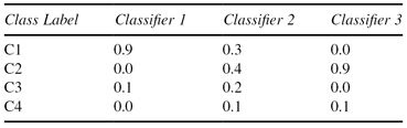
Each number in the above table describes the probability that a classifier predicts the class of a new sample as a corresponding class. For example, the probability that
Classifier 1 predicts
the class of X as C1 is 0.9.
When the ensemble combines predictions of each of them, as a combination method:
(a)
If the
simple sum
is used, which class is X classified as and why?
(b)
If the
weight sum
is used, which class is X classified as and why?
(c)
If the
rank-level fusion
is used, which class is X classified as and why?
10.
Suppose you have a drug discovery data set, which has 1950 samples and 100,000 features. You must classify chemical compounds represented by structural molecular features as active or inactive using ensemble learning. In order to generate diverse and independent classifiers for an ensemble, which ensemble methodology would you choose? Explain the reason for selecting that methodology.
11.
Which of the following is a fundamental difference between bagging and boosting?
(a)
Bagging is used for supervised learning. Boosting is used with unsupervised clustering.
(b)
Bagging gives varying weights to training instances. Boosting gives equal weight to all training instances.
(c)
Bagging does not take the performance of previously built models into account when building a new model. With boosting each new model is built based upon the results of previous models.
(d)
With boosting, each model has an equal weight in the classification of new instances. With bagging, individual models are given varying weights.
8.6 REFERENCES FOR FURTHER STUDY
Brown, G., Ensemble Learning, in
Encyclopedia of Machine Learning
, C. Sammut and Webb G. I., eds., Springer Press, New York, 2010.
“Ensemble learning refers to the procedures employed to train multiple learning machines and combine their outputs, treating them as a committee of decision makers.” The principle is that the committee decision, with individual predictions combined appropriately, should have better overall accuracy, on average, than any individual committee member. Numerous empirical and theoretical studies have demonstrated that ensemble models very often attain higher accuracy than single models. Ensemble methods constitute some of the most robust and accurate learning algorithms of the past decade. A multitude of heuristics has been developed for randomizing the ensemble parameters to generate diverse models. It is arguable that this line of investigation is rather oversubscribed nowadays, and the more interesting research is now in methods for nonstandard data.
Kuncheva, L. I.,
Combining Pattern Classifiers: Methods and Algorithms
, Wiley Press, Hoboken, NJ, 2004.
Covering pattern classification methods,
Combining Classifiers: Methods and Algorithms
focuses on the important and widely studied issue of combining several classifiers together in order to achieve an improved recognition performance. It is one of the first books to provide unified, coherent, and expansive coverage of the topic and as such will be welcomed by those involved in the area. With case studies that bring the text alive and demonstrate “real-world” applications it is destined to become an essential reading.
Dietterich, T. G., Ensemble Methods in Machine Learning, in
Lecture Notes in Computer Science on Multiple Classifier Systems
, Vol. 1857, Springer, Berlin, 2000.
Ensemble methods are learning algorithms that construct a set of classifiers and then classify new data points by taking a (weighted) vote of their predictions. The original ensemble method is Bayesian averaging, but more recent algorithms include error-correcting output coding, bagging, and boosting. This paper reviews these methods and explains why ensembles can often perform better than any single classifier. Some previous studies comparing ensemble methods are reviewed, and some new experiments are presented to uncover the reasons that Adaboost does not overfit rapidly.
9
CLUSTER ANALYSIS
Chapter Objectives
- Distinguish between different representations of clusters and different measures of similarities.
- Compare the basic characteristics of agglomerative- and partitional-clustering algorithms.
- Implement agglomerative algorithms using single-link or complete-link measures of similarity.
- Derive the K-means method for partitional clustering and analysis of its complexity.
- Explain the implementation of incremental-clustering algorithms and its advantages and disadvantages.
- Introduce concepts of density clustering, and algorithms Density-Based Spatial Clustering of Applications with Noise (DBSCAN) and Balanced and Iterative Reducing and Clustering Using Hierarchies (BIRCH).
- Discuss why validation of clustering results is a difficult problem.
Cluster analysis is a set of methodologies for automatic classification of samples into a number of groups using a measure of association so that the samples in one group are similar and samples belonging to different groups are not similar. The input for a system of cluster analysis is a set of samples and a measure of similarity (or dissimilarity) between two samples. The output from cluster analysis is a number of groups (clusters) that form a partition, or a structure of partitions, of the data set. One additional result of cluster analysis is a generalized description of every cluster, and this is especially important for a deeper analysis of the data set’s characteristics.
9.1 CLUSTERING CONCEPTS
Organizing data into sensible groupings is one of the most fundamental approaches of understanding and learning. Cluster analysis is the formal study of methods and algorithms for natural grouping, or clustering, of objects according to measured or perceived intrinsic characteristics or similarities. Samples for clustering are represented as a vector of measurements, or more formally, as a point in a multidimensional space. Samples within a valid cluster are more similar to each other than they are to a sample belonging to a different cluster. Clustering methodology is particularly appropriate for the exploration of interrelationships among samples to make a preliminary assessment of the sample structure. Human performances are competitive with automatic-clustering procedures in one, two, or three dimensions, but most real problems involve clustering in higher dimensions. It is very difficult for humans to intuitively interpret data embedded in a high-dimensional space.
Table
9.1
shows a simple example of clustering information for nine customers, distributed across three clusters. Two features describe customers: The first feature is the number of items the customers bought, and the second feature shows the price they paid for each.
TABLE 9.1.
Sample Set of Clusters Consisting of Similar Objects
| | Number of Items | Price |
| Cluster 1 | 2 | 1700 |
| 3 | 2000 | |
| 4 | 2300 | |
| Cluster 2 | 10 | 1800 |
| 12 | 2100 | |
| 11 | 2500 | |
| Cluster 3 | 2 | 100 |
| 3 | 200 | |
| 3 | 350 |
Customers in Cluster 1 purchase a few high-priced items; customers in Cluster 2 purchase many high-priced items; and customers in Cluster 3 purchase few low-priced items. Even this simple example and interpretation of a cluster’s characteristics shows that clustering analysis (in some references also called unsupervised classification) refers to situations in which the objective is to construct decision boundaries (classification surfaces) based on unlabeled training data set. The samples in these data sets have only input dimensions, and the learning process is classified as unsupervised.
Clustering is a very difficult problem because data can reveal clusters with different shapes and sizes in an n-dimensional data space. To compound the problem further, the number of clusters in the data often depends on the resolution (fine vs. coarse) with which we view the data. The next example illustrates these problems through the process of clustering points in the Euclidean two-dimensional (2-D) space. Figure
9.1
a shows a set of points (samples in a 2-D space) scattered on a 2-D plane. Let us analyze the problem of dividing the points into a number of groups. The number of groups N is not given beforehand. Figure
9.1
b shows the natural clusters bordered by broken curves. Since the number of clusters is not given, we have another partition of four clusters in Figure
9.1
c that is as natural as the groups in Figure 9.1b. This kind of arbitrariness for the number of clusters is a major problem in clustering.
Figure 9.1.
Cluster analysis of points in a 2D-space. (a) Initial data; (b) three clusters of data; (c) four clusters of data.
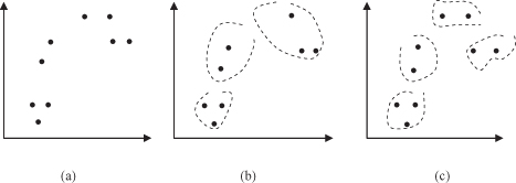
Note that the above clusters can be recognized by sight. For a set of points in a higher dimensional Euclidean space, we cannot recognize clusters visually. Accordingly, we need an objective criterion for clustering. To describe this criterion, we have to introduce a more formalized approach in describing the basic concepts and the clustering process.
An input to a cluster analysis can be described as an ordered pair (X,
s
), or (X,
d
), where X is a set of object descriptions represented with samples, and
s
and
d
are measures for similarity or dissimilarity (distance) between samples, respectively. Output from the clustering system is a partition Λ = {G
1
, G
2
, … , G
N
}, where G
k
, k = 1, … , N is a crisp subset of X such that
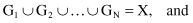
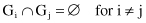
The members G
1
, G
2
, … , G
N
of Λ are called clusters. Every cluster may be described with some characteristics. In discovery-based clustering, both the cluster (a separate set of points in X) and its descriptions or characterizations are generated as a result of a clustering procedure. There are several schemata for a formal description of discovered clusters:
1.
Represent a cluster of points in an n-dimensional space (samples) by their centroid or by a set of distant (border) points in a cluster.
2.
Represent a cluster graphically using nodes in a clustering tree.
3.
Represent clusters by using logical expression on sample attributes.
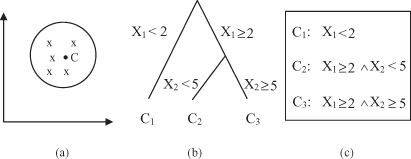
Figure
9.2
illustrates these ideas. Using the centroid to represent a cluster is the most popular schema. It works well when the clusters are compact or isotropic. When the clusters are elongated or non-isotropic, however, this schema fails to represent them properly.
Figure 9.2.
Different schemata for cluster representation. (a) Centroid; (b) clustering tree; (c) logical expressions.
The availability of a vast collection of clustering algorithms in the literature and also in different software environments can easily confound a user attempting to select an approach suitable for the problem at hand. It is important to mention that there is no clustering technique that is universally applicable in uncovering the variety of structures present in multidimensional data sets. The user’s understanding of the problem and the corresponding data types will be the best criteria in selecting the appropriate method. Most clustering algorithms are based on the following two popular approaches:
1.
hierarchical clustering, and
2.
iterative square-error partitional clustering.
Hierarchical techniques organize data in a nested sequence of groups, which can be displayed in the form of a dendrogram or a tree structure. Square-error partitional algorithms attempt to obtain the partition that minimizes the within-cluster scatter or maximizes the between-cluster scatter. These methods are nonhierarchical because all resulting clusters are groups of samples at the same level of partition. To guarantee that an optimum solution has been obtained, one has to examine all possible partitions of the N samples with n dimensions into K clusters (for a given K), but that retrieval process is not computationally feasible. Notice that the number of all possible partitions of a set of N objects into K clusters is given by:

So various heuristics are used to reduce the search space, but then there is no guarantee that the optimal solution will be found.
Hierarchical methods that produce a nested series of partitions are explained in Section 6.3, while partitional methods that produce only one level of data grouping are given with more details in Section 9.4. The next section introduces different measures of similarity between samples; these measures are the core component of every clustering algorithm.
9.2 SIMILARITY MEASURES
To formalize the concept of a similarity measure, the following terms and notation are used throughout this chapter. A sample
x
(or feature vector, observation) is a single-data vector used by the clustering algorithm in a space of samples X. In many other texts, the term pattern is used. We do not use this term because of a collision in meaning with patterns as in pattern-association analysis, where the term has a totally different meaning. Most data samples for clustering take the form of finite dimensional vectors, and it is unnecessary to distinguish between an object or a sample x
i
, and the corresponding vector. Accordingly, we assume that each sample x
i
∈ X, i = 1, … , n is represented by a vector x
i
= {x
i1
, x
i2
, … , x
im
}. The value m is the number of dimensions (features) of samples, while n is the total number of samples prepared for a clustering process that belongs to the sample domain X.