Structure and Interpretation of Computer Programs (67 page)
Read Structure and Interpretation of Computer Programs Online
Authors: Harold Abelson and Gerald Jay Sussman with Julie Sussman

Exercise 3.74.
Alyssa P. Hacker is designing a system to process signals coming from
physical sensors. One important feature she wishes to produce is a
signal that describes the
zero crossings
of the input signal.
That is, the resulting signal should be + 1 whenever the input signal
changes from negative to positive, - 1 whenever the input signal
changes from positive to negative, and 0 otherwise. (Assume that the
sign of a 0 input is positive.) For example, a typical input signal
with its associated zero-crossing signal would be
...
1 2 1.5 1 0.5 -0.1 -2 -3 -2 -0.5 0.2 3 4
...
...
0 0 0 0 0 -1 0 0 0 0 1 0 0
...
In Alyssa's system, the signal from the sensor is represented as a
stream
sense-data
and the stream
zero-crossings
is
the corresponding stream of zero crossings. Alyssa first writes a
procedure
sign-change-detector
that takes two values as
arguments and compares the signs of the values to produce an
appropriate 0, 1, or - 1. She then constructs her zero-crossing
stream as follows:
(define (make-zero-crossings input-stream last-value)
(cons-stream
(sign-change-detector (stream-car input-stream) last-value)
(make-zero-crossings (stream-cdr input-stream)
(stream-car input-stream))))
(define zero-crossings (make-zero-crossings sense-data 0))
Alyssa's boss, Eva Lu Ator, walks by and suggests that this program is
approximately equivalent to the following one, which
uses the generalized version
of
stream-map
from exercise
3.50
:
(define zero-crossings
(stream-map sign-change-detector sense-data <
expression
>))
Complete the program by supplying the indicated <
expression
>.
Exercise 3.75.
Unfortunately, Alyssa's zero-crossing detector in
exercise
3.74
proves to be insufficient, because the
noisy signal from the sensor leads to spurious zero crossings. Lem E.
Tweakit, a hardware specialist, suggests that Alyssa smooth the signal
to filter out the noise before extracting the zero crossings. Alyssa
takes his advice and decides to extract the zero crossings from the
signal constructed by averaging each value of the sense data with the
previous value. She explains the problem to her assistant, Louis
Reasoner, who attempts to implement the idea, altering Alyssa's program as
follows:
(define (make-zero-crossings input-stream last-value)
(let ((avpt (/ (+ (stream-car input-stream) last-value) 2)))
(cons-stream (sign-change-detector avpt last-value)
(make-zero-crossings (stream-cdr input-stream)
avpt))))
This does not correctly implement Alyssa's plan.
Find the bug that Louis has installed
and fix it without changing the structure of the program. (Hint: You
will need to increase the number of arguments to
make-zero-crossings
.)
Exercise 3.76.
Eva Lu Ator has a criticism of Louis's approach in
exercise
3.75
. The program he wrote is not modular,
because it intermixes the operation of smoothing with the
zero-crossing extraction. For example, the extractor should not have
to be changed if Alyssa finds a better way to condition her input
signal. Help Louis by writing a procedure
smooth
that takes a
stream as input and produces a stream in which each element is the
average of two successive input stream elements. Then use
smooth
as a component to implement the zero-crossing detector in a
more modular style.
The
integral
procedure at the end of the preceding section shows
how we can use streams to model signal-processing systems that contain
feedback loops. The feedback loop for the adder shown in
figure
3.32
is modeled by the fact that
integral
's
internal stream
int
is defined in terms of itself:
(define int
(cons-stream initial-value
(add-streams (scale-stream integrand dt)
int)))
The interpreter's ability to deal with such an implicit definition
depends on the
delay
that is incorporated into
cons-stream
. Without this
delay
, the interpreter could not
construct
int
before evaluating both arguments to
cons-stream
, which would require that
int
already be defined.
In general,
delay
is crucial for using streams to model
signal-processing systems that contain loops. Without
delay
,
our models would have to be formulated so that the inputs to any
signal-processing component would be fully evaluated before the output
could be produced. This would outlaw loops.
Unfortunately, stream models of systems with loops
may require uses of
delay
beyond the “hidden”
delay
supplied by
cons-stream
. For instance,
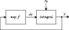
figure
3.34
shows a signal-processing system for
solving the
differential equation
d
y
/
d
t
=
f
(
y
) where
f
is a given
function. The figure shows a mapping component, which
applies
f
to its input signal, linked in a feedback loop to an
integrator in a manner very similar to that of the analog computer
circuits that are actually used to solve such equations.
 |
Assuming we are given an initial value
y
0
for
y
, we
could try to model this system using the procedure
(define (solve f y0 dt)
(define y (integral dy y0 dt))
(define dy (stream-map f y))
y)
This procedure does not work, because in the first line of
solve
the call to
integral
requires that the input
dy
be
defined, which does not happen until the second line of
solve
.
On the other hand, the intent of our definition does make sense,
because we can, in principle, begin to generate the
y
stream
without knowing
dy
. Indeed,
integral
and many other
stream operations have properties similar to those of
cons-stream
, in that we can generate part of the answer given only
partial information about the arguments. For
integral
, the
first element of the output stream is the specified
initial-value
. Thus, we can generate the first element of the output
stream without evaluating the integrand
dy
. Once we know the
first element of
y
, the
stream-map
in the second line of
solve
can begin working to generate the first element of
dy
, which will produce the next element of
y
, and so on.
To take advantage of this idea, we will redefine
integral
to
expect the integrand stream to be a
delayed argument
.
Integral
will
force
the integrand to be evaluated only when it
is required to generate more than the first element of the output stream:
(define (integral delayed-integrand initial-value dt)
(define int
(cons-stream initial-value
(let ((integrand (force delayed-integrand)))
(add-streams (scale-stream integrand dt)
int))))
int)
Now we can implement our
solve
procedure by delaying the
evaluation of
dy
in the definition of
y
:
71
(define (solve f y0 dt)
(define y (integral (delay dy) y0 dt))
(define dy (stream-map f y))
y)
In general, every caller of
integral
must now
delay
the
integrand argument. We can demonstrate that the
solve
procedure
works by approximating
e
≈ 2.718 by computing the value at
y
= 1 of the solution to the differential equation
d
y
/
d
t
=
y
with
initial condition
y
(0) = 1:
(stream-ref (solve (lambda (y) y) 1 0.001) 1000)
2.716924
Exercise 3.77.
The
integral
procedure used above was analogous to the
“implicit” definition of the infinite stream of integers in
section
3.5.2
. Alternatively, we can give a
definition of
integral
that is more like
integers-starting-from
(also in section
3.5.2
):
(define (integral integrand initial-value dt)
(cons-stream initial-value
(if (stream-null? integrand)
the-empty-stream
(integral (stream-cdr integrand)
(+ (* dt (stream-car integrand))
initial-value)
dt))))
When used in systems with loops, this procedure has the same problem
as does our original version of
integral
. Modify the procedure
so that it expects the
integrand
as a delayed argument and hence
can be used in the
solve
procedure shown above.
Exercise 3.78.
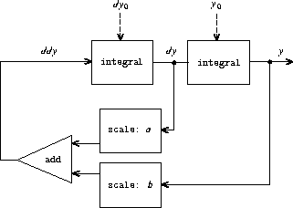 |
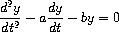
Consider the problem of designing a signal-processing system to study
the homogeneous second-order linear differential equation
The output stream, modeling
y
, is generated by a network that
contains a loop. This is because the value of
d
2
y
/
d
t
2
depends
upon the values of
y
and
d
y
/
d
t
and both of these are determined by
integrating
d
2
y
/
d
t
2
. The diagram we would like to encode is
shown in figure
3.35
. Write a procedure
solve-2nd
that
takes as arguments the constants
a
,
b
, and
d
t
and the initial
values
y
0
and
d
y
0
for
y
and
d
y
/
d
t
and generates the
stream of successive values of
y
.