Structure and Interpretation of Computer Programs (68 page)
Read Structure and Interpretation of Computer Programs Online
Authors: Harold Abelson and Gerald Jay Sussman with Julie Sussman

Exercise 3.79.
Generalize the
solve-2nd
procedure of exercise
3.78
so
that it can be used to solve general second-order differential
equations
d
2
y
/
d
t
2
=
f
(
d
y
/
d
t
,
y
).
Exercise 3.80.
A
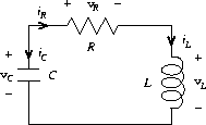
series RLC circuit
consists of a resistor, a capacitor, and an
inductor connected in series, as shown in figure
3.36
.
If
R
,
L
, and
C
are the resistance, inductance, and capacitance,
then the relations between voltage (
v
) and current (
i
)
for the three components are described by the equations

and the circuit connections dictate the relations

Combining these equations shows that the state of the circuit
(summarized by
v
C
, the voltage across the capacitor, and
i
L
, the
current in the inductor)
is described by the pair of differential equations

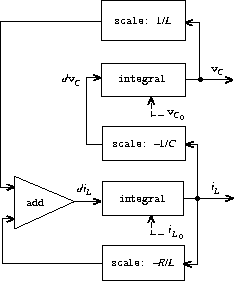
The signal-flow diagram representing this system of differential
equations is shown in figure
3.37
.
 |
 |
Write a procedure
RLC
that takes as arguments the parameters
R
,
L
, and
C
of the circuit and the time increment
d
t
. In a
manner similar to that of the
RC
procedure of
exercise
3.73
,
RLC
should produce a procedure
that takes the initial values of the state variables,
v
C
0
and
i
L
0
, and produces a pair (using
cons
) of the streams of
states
v
C
and
i
L
. Using
RLC
, generate the pair of
streams that models the behavior of a series RLC circuit with
R
= 1
ohm,
C
= 0.2 farad,
L
= 1 henry,
d
t
= 0.1 second, and initial
values
i
L
0
= 0 amps and
v
C
0
= 10 volts.
The examples in this section illustrate how the explicit use of
delay
and
force
provides great programming flexibility, but the
same examples also show how this can make our programs more complex.
Our new
integral
procedure, for instance, gives us the power to
model systems with loops, but we must now remember that
integral
should be called with a delayed integrand, and every procedure that
uses
integral
must be aware of this. In effect, we have created
two classes of procedures: ordinary procedures and procedures that
take delayed arguments. In general, creating separate classes of
procedures forces us to create separate classes of higher-order
procedures as well.
72
One way to avoid the need for two different classes of procedures is
to make all procedures take delayed arguments. We could adopt a model
of evaluation in which all arguments to procedures are automatically
delayed and arguments are forced only when they are actually needed
(for example, when they are required by a primitive operation). This
would transform our language to use normal-order evaluation, which we
first described when we introduced the substitution model for
evaluation in section
1.1.5
. Converting to
normal-order evaluation provides a uniform and elegant way to simplify
the use of delayed evaluation, and this would be a natural strategy to
adopt if we were concerned only with stream processing. In
section
4.2
, after we have studied the evaluator, we
will see how to transform our language in just this way.
Unfortunately, including delays in procedure calls wreaks havoc with
our ability to design programs that depend on the order of events,
such as programs that use assignment, mutate data, or perform input or
output. Even the single
delay
in
cons-stream
can cause
great confusion, as illustrated by exercises
3.51
and
3.52
. As far as anyone knows, mutability and delayed
evaluation do not mix well in programming languages, and devising ways
to deal with both of these at once is an active area of research.
As we saw in section
3.1.2
, one of the
major benefits of introducing assignment is that we can increase the
modularity of our systems by encapsulating, or “hiding,” parts of
the state of a large system within local variables. Stream models can
provide an equivalent modularity without the use of assignment. As an
illustration, we can reimplement the Monte Carlo estimation of π,
which we examined in section
3.1.2
, from a
stream-processing point of view.
The key modularity issue was that we wished to hide the internal state
of a random-number generator from programs that used random numbers.
We began with a procedure
rand-update
, whose successive values
furnished our supply of random numbers, and used this to produce a
random-number generator:
(define rand
(let ((x random-init))
(lambda ()
(set! x (rand-update x))
x)))
In the stream formulation there is no random-number generator
per
se
, just a stream of random numbers produced by successive calls to
rand-update
:
(define random-numbers
(cons-stream random-init
(stream-map rand-update random-numbers)))
We use this to construct the stream of outcomes of the Cesàro
experiment performed on consecutive pairs in the
random-numbers
stream:
(define cesaro-stream
(map-successive-pairs (lambda (r1 r2) (= (gcd r1 r2) 1))
random-numbers))
(define (map-successive-pairs f s)
(cons-stream
(f (stream-car s) (stream-car (stream-cdr s)))
(map-successive-pairs f (stream-cdr (stream-cdr s)))))
The
cesaro-stream
is now fed to a
monte-carlo
procedure,
which produces a stream of estimates of probabilities. The results
are then converted into a stream of estimates of π. This version
of the program doesn't need a parameter telling how many trials to
perform. Better estimates of π (from performing more experiments)
are obtained by looking farther into the
pi
stream:
(define (monte-carlo experiment-stream passed failed)
(define (next passed failed)
(cons-stream
(/ passed (+ passed failed))
(monte-carlo
(stream-cdr experiment-stream) passed failed)))
(if (stream-car experiment-stream)
(next (+ passed 1) failed)
(next passed (+ failed 1))))
(define pi
(stream-map (lambda (p) (sqrt (/ 6 p)))
(monte-carlo cesaro-stream 0 0)))
There is considerable modularity in this approach, because we still
can formulate a general
monte-carlo
procedure that can deal with
arbitrary experiments. Yet there is no assignment or local state.
Exercise 3.81.
Exercise
3.6
discussed generalizing the random-number generator to
allow one to reset the random-number sequence so as to produce
repeatable sequences of “random” numbers. Produce a stream
formulation of this same generator that operates on an input stream of
requests to
generate
a new random number or to
reset
the
sequence to a specified value and that produces the desired stream of
random numbers. Don't use assignment in your solution.
Exercise 3.82.
Redo exercise
3.5
on Monte Carlo
integration in terms of streams. The stream version of
estimate-integral
will not have an argument telling how many trials
to perform. Instead, it will produce a stream of estimates based on
successively more trials.
Let us now return to the issues of objects and state that were raised
at the beginning of this chapter and examine them in a new light. We
introduced assignment and mutable objects to provide a mechanism for
modular construction of programs that model systems with state.
We constructed computational
objects with local state variables and used assignment to modify these
variables. We modeled the temporal behavior of the objects in the
world by the temporal behavior of the corresponding computational
objects.